Introduction
Image mosaicing generally contains image pre-processing, image registration and image mosaic [3].The aim of pre=processing is to simplify the difficulties of image registration to make some replication change and transformation od coordinates on original image. The core problem of image registration is to find out a space variation and register the coordinate points of overlapping parts between images. The main process of image mosaic includes: mosaic adjoining images’ registering areas, get rid of accumulated mistakes made in the process of overall mosaic and distortion phenomenon in image overlapping area, and draw and output mosaic image.
The image mosaicing procedure generally includes three steps. First, we register input images by estimating the homography, which relates pixels in one frame to their corresponding pixels in another frame. Second, we warp input frames according to the estimated homography so that their overlapping regions align. Finally, we paste the warped images and blend them on a common mosaicing surface to build the mosaic result.
Image Registration
Image registration is the establishment of correspondence between the images of same scene. It is a process of aligning two images acquire by same or different sensors, at different time or from different viewpoint. To register images, we need to determine geometric transformation that aligns images with respect to the reference image [1].
Steps involved in the registration process as in [2] are as follow:
- Feature Detection: Salient and distinctive objects in both reference and sensed images are detected.
- Feature Matching: The correspondence between the features in the reference and the sensed image established.
- Transform Model Estimation:The type and parameters of the so-called mapping functions, aligning the sensed image with the reference image, are estimated.
- Image Resampling: The sensed image is transformed by means of the mapping functions.
Image Blending
It is the final step to blend the pixels colours (or intensity) in the overlapped region to avoid the seams. Simplest available form is to use feathering, which uses weighted averaging colour values to blend the overlapping pixels.
Our main focus is on the first step of image registration process of feature detection. Features are the distinct elements in two images that are to be matched. The image mosaicing methods can be loosely classified based on the following classes as given in [3].
- Algorithms that use pixel values directly, e.g., correlation methods.
- Algorithms that use frequency domain, e.g., Fast Fourier transform methods.
- Algorithms that use low level features like edges and corners detection.
- Algorithms that use high level features like identified parts of image objects, etc.
Proposed Work
The proposed method aims in detecting overlapping portion for extracting matching points. The overlapping regions are determined using gradient based dominant edge extraction and invariant moments. In the deduced region, the SIFT (Shift Invariant Feature Transform) features are extracted to determine the matching features. The registration is carried on with RANSAC (Random Sample Consensus) algorithm and final output mosaic is obtained by warping the images [4].
Selection of Matching Regions
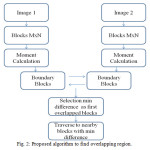
Basically, proposed algorithm is the optimization of pre-processing step of image mosaicing (i.e., to find overlapping region). As in the previous section, it is found that with the increase of number of blocks of images also increase the time complexity. This complexity can be reduced by only considering the boundary blocks of both images first. Then moment difference values are calculated using standard deviation method instead of sum of absolute moment difference. Minimum difference value is selected for image blocks as overlapping region. After that, there is a need to traverse through the neighborhood blocks in both the images for continuous common region with some threshold value for blocks match. So in short the process will be as follows,
- Moment invariants calculation of all blocks.
- Compare moment difference values of boundary blocks of both images.
- Select with minimum value for overlapping blocks.
- Set the threshold value.
- Traverse through neighbor blocks.
Fig.2 is the flow chart of the proposed algorithm.
Edge Detection
One way to reduce the time complexity is to use only the dominant information from images like edges. This could significantly reduce the matching cost. Traditional edge detection methods like sobel, prewitt and Roberts operators are applied in determining the edges. These approaches failed to yield better results under varying environmental and illumination conditions. Gradient based edge detection produced better results for natural color images [4].
An algorithm uses a two-dimensional implementation of the Canny edge detection method to detect and localize significant edges in the input image [6]. The first step in the gradient-based edge detection is estimation of the underlying gradient function. This is achieved by convolution of the input image with an appropriately chosen filter. The filter used is a two-dimensional Canny filter, which is the directional derivative of a two-dimensional Gaussian distribution defined by
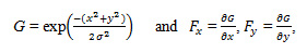
Where x and y denote absolute pixel coordinates. The advantage of using such a filter is that it inherently smoother the image while estimating its gradient, thereby reducing the range of scales over which intensity changes in the input image take place [6P]. The overall size of each filter, Fx and Fy, is a function of the desired edge scale and the image resolution.
σ= gradient length scale (pixels) = (desired edge scale / image resolution)
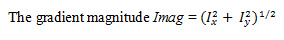
The next step in the Canny edge detection method is to thin the contours of the gradient image, Imag, and suppress (i.e. discard) any contours of magnitude less than a given threshold [8].
After determining the dominant edges from the images, images are partitioned into equal sized blocks and compared against each other for finding the similarity [4].
Calculation of Moment Invariants
After determining the dominant edges from the images, images are partitioned into equal sized blocks and compared against each other for finding the similarity [4]. The moment invariants are moment-based descriptors on shapes, which are invariant under general translational, rotational, scaling transformation. The moments of a binary image f(i,j) are given by eq. (3.1).
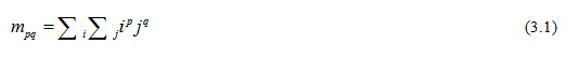
where p and q define the order of the moment. Zero order moment are used to represent the binary object area. Second-order moments represents the distribution of matter around the center. The invariant moments of lower order are enough for most registration tasks on remotely sensed image matching. If (x, y) is a digital image, then the central moments are defined by the Eq. (3.2).

Moments ηij where i + j >2 can be constructed to be invariant to both translation and changes in scale by dividing the corresponding central moment by the properly scaled (00)th moment, using the following formula.
From moments ηij seven Invariant moments are calculated with Equations 3.4 to 3.10.
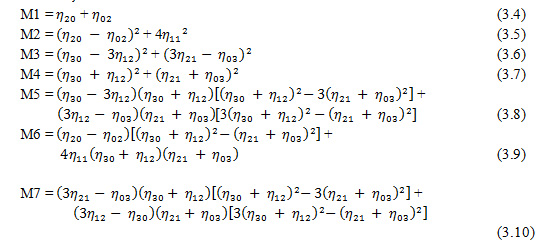
The seven invariant moments M1 to M7 mentioned in from Eq. (3.4) to (3.10) are typical unchanged properties of images under rotation, scale and translation. After determining the dominant edges of the images, the images are partitioned into equal sized blocks. The standard deviation of difference between the moment values can be obtained from input images. The blocks with the minimum difference value is considered and taken up as the matching regions for the following steps of extracting SIFT features [4].
Standard Deviation of Moment Difference
Generally seven moment values of order 3 of image are used in the analysis in the field of image processing. As we seen in the previous section, seven moment invariants were calculated.
Let say we have moments M and N for two images as given below:
M = [ M1 M2 M3 M4 M5 M6 M7 ]
N = [ N1 N2 N3 N4 N5 N6 N7 ]
Then difference set can be given as
D = M – N
= [ M1-N1 M2-N2 ———– M7-N7 ]
= [ D1 D2 ——— D7 ] (3.11)
After that mean value is calculated as
Mean = SUM (ABS (D)) / 7 (3.12)
This Mean value is substracted from the D as deviation
Dev = [ D – Mean ]
= [ D1-Mean ———— D7-Mean ]
= [ Dev1 Dev2 ————- Dev7 ] (3.13)
Based on these deviation values, variance is calculated as
Variance σ2 = / 7
= [ + + ………… + ] / 7 (3.14)
Standard Deviation of moment invariants difference is the square-root of Variance as
Selection Overlapping Blocks
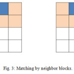
After finding the minimum difference value for first overlapped blocks, further region can be obtain by traversing through the nearby blocks by comparison of moment difference values to some minimum threshold value.
SIFT Feature Extraction
SIFT algorithm is used for extracting the features from the matching regions. It consists of four steps namely scale-space extrema detection, keypoint localization, orientation assignment and a keypoint descriptors [4]. SIFT Algorithm is Scale Invariant Feature Transform. SIFT is an corner detection algorithm which detects features in an image which can be used to identify similar objects in other images [3]. SIFT produces key-point-descriptors which are the image features. When checking for an image match two set of key-point descriptors are given as input to the Nearest Neighbor Search (NNS) and produces a closely matching key-point descriptors. SIFT has four computational phases which includes: Scale-space construction, Scale-space extrema detection, key-point localization, orientation assignment and defining key-point descriptors [3].
The first phase identifies the potential interest points. It searches over all scales and image locations by using a difference-of Gaussian function. For all the interest points so found in phase one, location and scale is determined. Key-points are selected based on their stability. A stable key-point should be resistant to image distortion. In Orientation assignment SIFT algorithm computes the direction of gradients around the stable key-points. One or more orientations are assigned to each key-point based on local image gradient directions. For a set of input frames SIFT extracts features [3].
Scale Invariant Feature Transform (SIFT) consists of four stages as below:
- Scale-space extrema detection: The first stage of computation searches over all scales and image locations. It is implemented efficiently by using a difference-of-Gaussian function to identify potential interest points that are invariant to scale and orientation.
- Keypoint localization: At each candidate location, a detailed model is fit to determine location and scale. Keypoints are selected based on measures of their stability.
- Orientation assignment: One or more orientations are assigned to each keypoint location based on local image gradient directions. All future operations are performed on image data that has been transformed relative to the assigned orientation, scale, and location for each feature, thereby providing invariance to these transformations.
- Keypoint descriptor: The local image gradients are measured at the selected scale in the region around each keypoint. These are transformed into a representation that allows for significant levels of local shape distortion and change in illumination.
The first stage used difference-of-Gaussian (DOG) function to identify potential interest points, which were invariant to scale and orientation. DOG was used instead of Gaussian to improve the computation speed.

Where * is the convolution operator, G(x, y, ) is a variable scale Gaussian, I(x, y) is the input image D(x, y, ) is Difference of Gaussians with scale k times. In the keypoint localization step, they are rejected the low contrast points and eliminated the edge response. Hessian matrix was used to compute the principal curvatures and eliminate the keypoints that have a ratio between the principal curvatures greater than the ratio. An orientation histogram was formed from the gradient orientations of sample points within a region around the keypoint in order to get an orientation assignment [7],[9],[10].
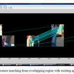
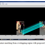
SIFT features where extracted only from the overlapped region in both images thus required less computation in the proposed algorithm.
Transformation Estimation
The RANdom SAmple Consensus (RANSAC) algorithm is a general parameter estimation approach designed to cope with a large proportion of outliers in the input data [9]. RANSAC is a resampling technique that generates candidate solutions by using the minimum number observations (data points) required to estimate the underlying model parameters. Unlike conventional sampling techniques that use as much of the data as possible to obtain an initial solution and then proceed to prune outliers, RANSAC uses the smallest set possible and proceeds to enlarge this set with consistent data points [9].
- Select randomly the minimum number of points required to determine the model parameters.
- Solve for the parameters of the model.
- Determine how many points from the set of all points fit with a predefined tolerance.
- If the fraction of the number of inliers over the total number points in the set exceeds a predefined threshold, re-estimate the model parameters using all the identified inliers and terminate.
- Otherwise, repeat steps 1 through 4 (maximum of N times).
The number of iterations, N, is chosen high enough to ensure that the probability p (usually set to 0.99) that at least one of the sets of random samples does not include an outlier. Let u represent the probability that any selected data point is inliers and v = 1 − u the probability of observing an outlier [9]. N iterations of the minimum number of points denoted m are required, where
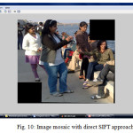
Experimental Results
Table 1: Moment invariant difference values calculated with existing approach (absolute difference)
|
data
|
|
|
|
1
|
2
|
3
|
4
|
5
|
6
|
7
|
8
|
9
|
10
|
11
|
12
|
13
|
14
|
15
|
16
|
|
1
|
8.4609
|
5.1627
|
5.6337
|
9.0123
|
8.3035
|
2.3650
|
7.6711
|
5.0450
|
8.2367
|
12.6924
|
9.3918
|
4.3539
|
8.7140
|
8.7838
|
3.9551
|
5.0912
|
|
2
|
4.8031
|
1.5049
|
1.9759
|
5.3545
|
4.6457
|
1.2928
|
4.0133
|
8.7028
|
4.5789
|
9.0346
|
5.7340
|
0.6961
|
5.0562
|
5.1260
|
7.6129
|
1.4335
|
|
3
|
6.9925
|
3.6943
|
4.1653
|
7.5439
|
6.8350
|
0.8966
|
6.2027
|
6.5134
|
6.7683
|
11.2240
|
7.9234
|
2.8855
|
7.2456
|
7.3154
|
5.4235
|
3.6228
|
|
4
|
0.5450
|
2.7532
|
2.2822
|
1.0964
|
0.3876
|
5.5509
|
0.2447
|
12.9609
|
0.3208
|
4.7765
|
1.4759
|
3.5620
|
0.7982
|
0.8679
|
11.8710
|
2.8246
|
|
5
|
6.8480
|
3.5498
|
4.0208
|
7.3994
|
6.6905
|
0.7521
|
6.0582
|
6.6579
|
6.6238
|
11.0795
|
7.7789
|
2.7410
|
7.1011
|
7.1709
|
5.5680
|
3.4783
|
|
6
|
1.1141
|
4.4123
|
3.9413
|
0.5627
|
1.2716
|
7.2100
|
1.9039
|
14.6200
|
1.3383
|
3.1174
|
0.1832
|
5.2211
|
0.8610
|
0.7912
|
13.5301
|
4.4838
|
|
7
|
3.6168
|
6.9150
|
6.4440
|
3.0654
|
3.7743
|
9.7127
|
4.4066
|
17.1227
|
3.8410
|
0.6147
|
2.6859
|
7.7238
|
3.3637
|
3.2939
|
16.0328
|
6.9865
|
|
8
|
0.7285
|
4.0267
|
3.5557
|
0.1771
|
0.8860
|
6.8244
|
1.5183
|
14.2344
|
0.9527
|
3.5029
|
0.2024
|
4.8355
|
0.4754
|
0.4056
|
13.1445
|
4.0982
|
|
9
|
2.5779
|
0.7203
|
0.2493
|
3.1293
|
2.4205
|
3.5180
|
1.7881
|
10.9280
|
2.3537
|
6.8094
|
3.5088
|
1.5291
|
2.8310
|
2.9008
|
9.8381
|
0.7918
|
|
10
|
4.8979
|
8.1961
|
7.7251
|
4.3465
|
5.0554
|
10.9939
|
5.6877
|
18.4038
|
5.1221
|
0.6665
|
3.9670
|
9.0050
|
4.6448
|
4.5750
|
17.3139
|
8.2676
|
|
11
|
2.7825
|
0.5157
|
0.0447
|
3.3339
|
2.6251
|
3.3134
|
1.9927
|
10.7234
|
2.5583
|
7.0140
|
3.7134
|
1.3245
|
3.0356
|
3.1054
|
9.6335
|
0.5871
|
|
12
|
3.7809
|
0.4827
|
0.9537
|
4.3323
|
3.6234
|
2.3150
|
2.9911
|
9.7250
|
3.5567
|
8.0123
|
4.7118
|
0.3261
|
4.0340
|
4.1038
|
8.6351
|
0.4112
|
|
13
|
2.2083
|
1.0899
|
0.6189
|
2.7597
|
2.0508
|
3.8876
|
1.4185
|
11.2976
|
1.9841
|
6.4397
|
3.1392
|
1.8987
|
2.4614
|
2.5312
|
10.2077
|
1.1614
|
|
14
|
2.8777
|
6.1759
|
5.7049
|
2.3263
|
3.0352
|
8.9736
|
3.6675
|
16.3836
|
3.1019
|
1.3537
|
1.9468
|
6.9847
|
2.6246
|
2.5548
|
15.2937
|
6.2474
|
|
15
|
5.8206
|
9.1188
|
8.6478
|
5.2692
|
5.9781
|
11.9165
|
6.6104
|
19.3265
|
6.0448
|
1.5891
|
4.8897
|
9.9276
|
5.5675
|
5.4977
|
18.2366
|
9.1903
|
|
16
|
0.7216
|
2.5766
|
2.1056
|
1.2730
|
0.5641
|
5.3743
|
0.0682
|
12.7843
|
0.4974
|
4.9531
|
1.6525
|
3.3854
|
0.9747
|
1.0445
|
11.6944
|
2.6481
|
|
Table 2: Moment invariant difference values calculated with proposed approach (standard deviation)
|
data
|
|
|
1
|
2
|
3
|
4
|
5
|
6
|
7
|
8
|
9
|
10
|
11
|
12
|
13
|
14
|
15
|
16
|
|
1
|
1.8354
|
3.4633
|
0.9025
|
4.1540
|
1.3492
|
2.0237
|
2.6276
|
2.7467
|
1.3685
|
2.0267
|
2.4882
|
0.6965
|
2.2762
|
2.3117
|
2.3176
|
2.9743
|
|
2
|
0.5025
|
1.4174
|
1.1360
|
2.0369
|
1.5346
|
0.6001
|
1.0146
|
0.8866
|
1.4117
|
1.1364
|
1.3845
|
1.4771
|
0.9425
|
0.2138
|
0.6687
|
1.1394
|
|
3
|
1.5341
|
3.2603
|
0.8621
|
3.7693
|
1.0967
|
1.8788
|
2.2628
|
2.7405
|
1.0846
|
1.6706
|
2.1656
|
0.7006
|
1.9593
|
2.0546
|
2.4954
|
2.7045
|
|
4
|
2.7762
|
1.4811
|
3.6829
|
2.4666
|
4.1922
|
2.4281
|
2.2480
|
3.0521
|
3.2539
|
2.7915
|
2.2668
|
4.1881
|
2.2231
|
2.1854
|
2.9256
|
1.7202
|
|
5
|
0.8202
|
1.7030
|
1.6033
|
2.2036
|
1.8733
|
0.5656
|
1.0652
|
0.6518
|
1.7739
|
1.4035
|
1.9140
|
1.8630
|
1.1986
|
1.0664
|
0.7202
|
1.3950
|
|
6
|
0.1907
|
1.2662
|
1.1033
|
1.7561
|
1.2432
|
0.7335
|
0.7376
|
1.0922
|
1.2407
|
0.7226
|
1.0033
|
1.2753
|
0.9391
|
0.7134
|
0.9032
|
0.8886
|
|
7
|
1.0267
|
1.6743
|
1.4677
|
1.9858
|
1.5532
|
1.3973
|
0.9128
|
2.1134
|
1.0630
|
0.5661
|
0.8785
|
1.6192
|
0.6881
|
1.0236
|
1.8814
|
1.3905
|
|
8
|
1.7103
|
2.1767
|
2.0937
|
2.5156
|
2.2836
|
1.8928
|
1.3227
|
2.6439
|
1.5342
|
0.2579
|
0.9751
|
2.3896
|
1.2741
|
1.4557
|
2.4207
|
1.5554
|
|
9
|
1.0625
|
1.3211
|
1.1492
|
1.6641
|
1.1778
|
0.4220
|
0.6514
|
1.0249
|
1.0964
|
1.0948
|
1.0430
|
1.2642
|
0.6550
|
1.0538
|
0.8005
|
0.8335
|
|
10
|
0.8917
|
2.1517
|
0.9843
|
2.7028
|
0.5262
|
1.2118
|
1.4111
|
1.7927
|
0.9205
|
1.2045
|
1.7486
|
0.9186
|
1.2990
|
1.3300
|
1.5882
|
1.2352
|
|
11
|
1.3989
|
0.1331
|
2.4541
|
1.2520
|
2.7253
|
1.4772
|
0.2706
|
2.2652
|
2.1409
|
1.4303
|
1.8034
|
2.7763
|
0.9457
|
0.7896
|
2.2198
|
0.5751
|
|
12
|
0.8934
|
0.7123
|
1.2954
|
1.0820
|
1.9634
|
1.1186
|
0.6023
|
1.7410
|
1.7551
|
1.0767
|
1.4678
|
2.2092
|
0.7253
|
0.7004
|
1.6556
|
0.2616
|
|
13
|
1.3704
|
2.7696
|
0.9818
|
3.5282
|
0.4019
|
1.6414
|
1.9493
|
2.5091
|
1.2512
|
1.4376
|
2.0011
|
0.9753
|
1.6456
|
1.7222
|
2.3572
|
2.3388
|
|
14
|
0.5864
|
1.5298
|
0.9159
|
2.0449
|
0.8455
|
0.9256
|
0.9907
|
1.3162
|
0.9587
|
0.5838
|
0.2911
|
1.0019
|
1.1087
|
0.8023
|
1.1894
|
1.0080
|
|
15
|
0.9003
|
1.6483
|
1.3383
|
2.0581
|
1.4026
|
1.2088
|
1.0136
|
1.7521
|
1.0261
|
0.6234
|
0.8423
|
1.5208
|
0.9698
|
1.0932
|
1.5276
|
1.2202
|
|
16
|
0.8636
|
1.5102
|
0.8017
|
1.9192
|
0.7835
|
0.9480
|
0.9399
|
1.5354
|
0.5255
|
0.6872
|
0.7383
|
1.0227
|
0.7466
|
0.9272
|
1.3624
|
1.1139
|
|
Performance Analysis
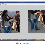
We have tested the algorithm on four different set of images for comparison as below:
Table 3: Comparison based on no. of features detected as matching points.
|
Data Set
|
No. of features detected
|
Percentage reduction
|
|
Existing
|
Proposed
|
SIFT
|
Existing
|
Proposed
|
|
Set 1
|
244
|
643
|
1128
|
78.37
|
43.00
|
|
Set 2
|
386
|
274
|
1517
|
74.56
|
81.96
|
|
Set 3
|
801
|
1193
|
4313
|
81.42
|
72.33
|
|
Set 4
|
207
|
427
|
1638
|
87.36
|
73.93
|
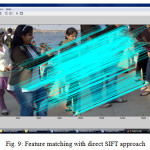
From the above table, we can see that number of features extracted is less than that of applying direct SIFT. Thus the SIFT will execute faster.
Table 4: Comparison based on time efficiency (second).
|
Data Set
|
Time Complexity of SIFT
|
Overall
|
Percentage reduction
|
|
Existing
|
Proposed
|
SIFT
|
Existing
|
Proposed
|
Existing
|
Proposed
|
|
Set 1
|
1.2324
|
1.0920
|
2.4336
|
3.4788
|
2.9796
|
49.36
|
55.13
|
|
Set 2
|
1.9344
|
1.6848
|
3.7596
|
7.7844
|
5.8344
|
48.55
|
55.19
|
|
Set 3
|
4.9608
|
3.1044
|
17.4877
|
20.9821
|
13.4161
|
71.63
|
82.24
|
|
Set 4
|
2.5740
|
2.2776
|
5.0388
|
11.4973
|
8.9077
|
48.91
|
54.79
|
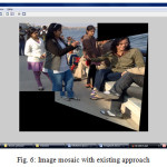
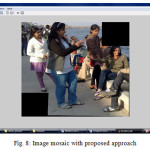
As seen in table 4, proposed algorithm is able to increase the computation speed that the existing algorithm. Also from the output mosaic, we can see the improvement on the quality of mosaic image is achieved.
Conclusion
With the experiment result and comparison between base and proposed approach, one can say that the quality of the image mosaicing is improve in the proposed algorithm then in the existing algorithm. Also the time complexity reduces to some extend with proposed approach then that in the existing approach. Overlapping region found with proposed approach is continuous and do not have any false match as that in the base approach. By such comparison, we can say that the proposed algorithm is better to find overlapping region which will reduce time for SIFT features extraction.
Acknowledgment
I am very grateful and would like to thank my guides Prof. Vikram Agrawal for his advice and continued support. Without him, it would have not been possible for me to complete this paper. I would like to thank all my friends for the thoughtful and mind stimulating discussion we had, which prompted us to think beyond the obvious.
References
- Manjusha Deshmukh, Udhav Bhosle, “A Survey of Image Registration”, International Journal of Image Processing (IJIP), Volume (5) : Issue (3) , 2011.
- Medha V. Wyawahare, Dr. Pradeep M. Patil, and Hemant K. Abhyankar, “Image Registration Techniques: An overview”, International Journal of Signal Processing, Image Processing and Pattern Recognition, Vol. 2, No.3, September 2009.
- Hemlata Joshi, Mr. Khomlal Sinha, “A Survey on Image Mosaicing Techniques”, International Journal of Advanced Research in Computer Engineering & Technology (IJARCET) Volume 2, Issue 2, February 2013.
- A.Annis Fathima, R. Karthik, V. Vaidehi, “Image Stitching with Combined Moment Invariants and SIFT Features”, Procedia Computer Science 19 ( 2013 ) 420 – 427.
CrossRef
- Udaykumar B Patel, Hardik N Mewada, “Review of Image Mosaic Based on Feature Technique”,International Journal of Engineering and Innovative Technology (IJEIT) Volume 2, Issue 11, May 2013.
- Hetal M. Patel, Pinal J. Patel, Sandip G. Patel, “Comprehensive Study And Review Of Image Mosaicing Methods”, International Journal of Engineering Research & Technology (IJERT), Vol. 1, Issue 9, November- 2012.
- M.M. El-gayar, H. Soliman, N. meky, “A comparative study of image low level feature extraction algorithms”, Egyptian Informatics Journal (2013) 14, 175–181.
CrossRef
- John J. Oram, James C. McWilliams, Keith D. Stolzenbach, “Gradient-based edge detection and feature classification of sea-surface images of the Southern California Bight”, Remote Sensing of Environment 112 (2008) 2397–2415.
CrossRef
- Konstantinos G. Derpanis, “Overview of the RANSAC Algorithm”, kosta@cs.yorku.ca, Version 1.2, May 13, 2010.
- David G. Lowe, “Distinctive Image Features from Scale-Invariant Keypoints”, Computer Science Department, University of British Columbia, Vancouver, B.C., Canada. (Accepted for publication in the International Journal of Computer Vision, 2004).

This work is licensed under a Creative Commons Attribution 4.0 International License.
 and Dilipsinh Bheda2
![Fig 1: Basic method of image mosaicing [6].](http://www.computerscijournal.org/wp-content/uploads/2017/02/Vol10_No1_Opt_Vik_Fig1-150x150.jpg)