Introduction
The expression “remote sensing satellites” is also called as the “aerial photography” regard as the depiction. The main research focused on the evolution of remote sensing satellites in four decades i.e., 1960-2010. Detecting the portraits of the huge plane from expanded partitions utilized airborne picture making and they utilized to grab the pictures.1 Remote sensing systems came into the photography and they have been fetched in satellites for depiction obtaining. To compare with planes, satellites cover2 more surface regions and there are widely utilized.
Remotely detected symbolism from satellites3 – investigate and upgraded with PCs – made it conceivable to recognize and screen these progressions. Only some groups are exceptional with the term remote sensing.
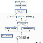
Remote satellites continuously obtaining high-resolution pictures of the earth’s surface on the base stations. Data will take care of base stations in running several partitions stepwise. These partitions process the data. After gathering data, data is preprocessing so as to eliminate the noisy elements in the data to obtain high throughput. The data transformed into pictures for the purpose of being comprehensible formats and these images can be analyzed. By utilizing parameters by pertaining the threshold provisions to the depictions will partition the picture into the number of blocks which can be analyzed easily processing in making a decision and promoting. Then we analyzed the predicted regions from the land surface.
The framework can be divided into block map and evaluation can be characterized with the help of flow chart.
Related Work
RS (Remote sensors) is utilized for ground observatory will stream the continuous data andcreates an extent of data. The researcher implemented diverse areas of applications in satellite remote sensing data, for instance, the gradient based edge detection,4 change, identification and so on. The continuous real time streaming data5 with high speed or the huge extent of data available in the form of big data which lead to many challenges? In this regard, the transformation of the sensor data from remote places are difficult to scientific understanding is a challenging task. Satellite remote sensing is utilizing of various technologies to constructscrutiny and dimensions of destination that is usually recognizable to the stripped eye. The technologies in remote sensing are classified as, radar, thermal, seismic, sonar, LiDAR, electric field sensing, GPS and infrared radiation. The remote sensing satellites will export the data in the form of offline and online real time data.
Many researchers developed models based on satellite data for predicting coastline analysis and erosion. For instance, for the change rates of shoreline, coastal corrosion and creation in coastal area6 utilized satellite data. GIS tools7 are used to analyze multi sequential remote sensing data from 1976 to 2000 and twenty scenes are taken for the varying model of accumulation and corrosion of the sub aerial delta of the Yellow River. The aerial photographs in black and white8 are utilized to estimating the changing rate in shoreline at USA Neuse River Estuary. Space simulation9 is initiating a novel mode of perceptive the geographical space which includes the dynamic processes in the space analysis.
Framework
Evolution Methods:
Dataset
Dataset is utilized in this work from “European space agency” which contains the number of tasks that are executed in the earlier period. And also took the necessary data for implementation and to examine the complex parameters for evaluation. After verifying these datasets will be added to the description. We classified these datasets into three main fields. The entire products are classified beneath of Advanced Synthetic Aperture Radar (ASAR).
Table 1: Data set of three major domains
| Domain |
/Dataset Details |
I/P Dataset Details |
Final Dataset Output |
| ASA_APM |
Alternating |
APM uses Range-Doppler Algorithm |
ASA_APM. XT |
| |
Polarization Mode |
used to derive higher-level products for SAR image quality assessment, calibration, and interferometric applications, |
converted to Image |
| ASA_IMM |
Image Mode
Medium Resolution
Image |
IMM uses
Covers a continuous area along the imaging swath and features an
ENL
(radiometric resolution) good enough for ice applications. |
ASA_IMM.XT converted to Image |
| ASA_GM1 |
Global Monitoring Image mode Product |
GM1 is processed to approximately 1 km resolution using the SPECAN algorithm |
ASA_GM1.XT converted to Image |
Category 1: Agency of European
ASAR product optional domain is APM (Alternating Polarization Mode) and it includes both Co-registered pictures belongs to three divergence amalgamation, secondary forms (VV and VH
HH and VV, HH and HV). In accumulation, the result utilizes the Range Doppler (RD) algorithm and preprocessing data parameters accessible. It can be activated to infer addedanimated items for SAR account superior appraisal, alignment, and interferon metric applications, if accustomed for the device attainment. The entire products will be in the structureof (.N1) extension categorizer design.
Preprocessing data: In this phase, cleaning the data for removing the unwanted elements. Theauthentic preprocessing techniques consist of header analysis, and these datasets having will.
HAN extension files. Give dataset is input to header analysis and it converting the dataset into picture format. For every time, it will carry on producing the set of documents that sustain the data retrieval.
Han documentation contains investigation and restrictions of the datasets. This documentation contains size, largeness and magnitude in pixels, dimensions and constraints like SPH indicators, etc. After header observation completed the properties of the datasets are able to understand and the dimensions of the datasets will be utilized for partitioning the picture into an amount of chunks.
Full resolution pictures of the dataset are .N1 form in .XT documents. The information is set up to be export in the form of understandable for humans, which looks like GeoTIFF, TIFF picture formats. Preferring any of the result’s format (for our experiment results we utilized TIFF) and sending the picture in needed directory file. A fundamental fault occurs if the time concerns and continuous without coordinating dataset. Beside the picture, it furthermore generates the accurate restrictions of the datasets.
Domain 2: Resolution Image Mode Medium
When the device was in picture mode the data accumulated at Level zero ASAR-IMM created. By comparing with ASA_IMP, this result has lesser resolution but elevated the radiometric resolution which is adequate for ice applications which apply to a continuous area close to the imaging swath and features a radiometric resolution (ENL). Preprocessing is same as the domain 1.
Domain 3: Image in Global Monitoring Mode
When the device was in global monitoring mode the data accumulated at Level zero ASAR-GM1 created. Each item covers an entire trajectory. The research work includes slant range to land modifications. Standard for ASAR Global Monitoring Mode is the strip-line product. By utilizing the SPECAN algorithm it processed to one km resolution approximately.
Methodology
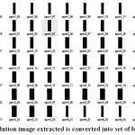
In our experiment results the image which is acquired from the dataset and partitioning image into tiny chunks in analyzing the geometric parameters. The partition is done due to come across the precise information. For every chunk, identifying the statistical parameters and assessment analysis is prepared from blocks. In our work, every image is partitioned into 20 blocks; these blocks are utilized for analysis accurate and easy.
The bunch of chunks derived from the picture will be using as input for the proposed algorithm. The algorithm acquires every chunk of the picture and updates the image list. This list is utilized diverse methods and functions for the purpose of analyze the statistical parameters of every chunk. For every picture chunk, the algorithm determines absolute difference, mean, standard deviation, etc.
For estimating the decision analysis process, the major parameters are:
Xi (Mean) 2. SD (Standard Deviation) 3. AD (Absolute difference) The variables and parameters utilized in our proposed algorithms.
Fixed size chunks of Picture are B1, B2, B3, B4, B5 … BN \.
Number of lines in the Image = NR.
Number of pixels in every line = NSR
Picture chunk size =
Total number of chunks in the picture = N ( N =NR ×NSR)
BS
Mean of model values of chunk B I = X Bi where i = {1, 2, 3, 4 . . . N}. Summation of all values of the chunk B i /the size of chunk = X Bi SD of sample values of chunk Bi. = SD Bi AB between X Bi and SD Bi = Abs_Diff
| X Bi − SD Bi | = Abs Diff
Total chunks mean Bi / the total number of chunks = Centric mean
By means of the above mention limitations, the subsequent will help in constructing the provisions and decision making.
The upper limit mean from mean of chunks is known as Maximum mean The maximum SD from SD of the chunks is known as Max SD. Maximum AD from AD of the chunks is known as Max AD Minimum AD from AD of the chunks is known as Min AD. Mean of all the chunks /Number of chunks = Centric mean
Table 2: Maximum and minimum of parameters
| Product/ Dataset |
Max_mean |
Min_mean |
Max_std |
Min_std |
Max_abs diff |
Min_abs diff |
| ASA_APM |
43.317369 |
1.8653104 |
10.448858 |
0.3913097 |
0.3913097 |
1.4093138 |
| ASA_IMM |
126.60508 |
0.6163557 |
40.749409 |
0.0604999 |
85.855666 |
0.1300828 |
| ASA_GM1 |
76.229318 |
2.626605 |
33.132327 |
0.6374876 |
48.503959 |
1.9891174 |
SD of all the chunks = Centric SD
Number of chunks
For simplifying the restrictions, the in detail conditions are identified. Those:
Mean less than Centric mean = MLCM
Mean greater than centric mean = MGCM
SD less than centric SD = SLCS
SD greater than centric SD = SGCS
AD less than centric AD = ALCA
AD greater than centric AD = AGCA
In our approach, we build the following laws for detection of the region
Centric mean >=Mean of Bi
Centric SD <= SD of Bi
AD of Bi <= Centric AD For every (Bi) {
If (law1 == true and law2 == true) Condition_Bi = earth
Else if (law1 == false andlaw2 == false) Condition_Bi = ocean
Else {
If (law3 == false and law1 == false))
Condition_Bi = ocean
Else
Condition_Bi = earth}
}
For identifying the earth chunks
Centric mean >= Mean of Bi
SD of Bi >= Centric SD
Centric mean >= Mean of Bi
AD of Bi > Centric AD
Centric mean < Mean of Bi
AD of Bi > Centric AD
For identifying the ocean chunks
Centric mean < Mean of Bi
SD of Bi < Centric SD
AD of Bi > Centric AD
Visualization of Data
After applying the above rules by making the blocks are able to understand that whether the blocks belong to land or sea regions. In our implementation, we take csv file belongs to the land blocks and sea blocks for the better visualization of data. For this, we utilized the python programming and done visualization for the acquired chunks based on the mean of the chunks. Packages in python programming are pandas, Numpy, matplotlib and seaborne which are utilizing for statistical analysis and understandable visualization.
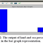
For example, the land and sea percentages for domain Alternating Polarization Medium are
Percentage of the Land is 83.3710954415.
Percentage of the Sea is 16.6289045585.
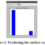
Analysis of Performance
We estimate the performance of the proposed method by increasing the number of chunks size and predicting the surface area region of land area or sea area.
Table 3: Number of blocks of each dataset
| S. No |
Product Domain |
Product/ Dataset Number |
No. of blocks |
| 1 |
ASA_AMP |
10 |
10*20=200 |
| 2 |
ASA_IMM |
10 |
200 |
| 3 |
ASA_GM1 |
10 |
200 |
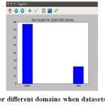
Table 4: The land and sea percentages of the surface area detected for three domains when a number of blocks considered are 200 and datasets number is 10.
| Domain/Product |
Number of blocks |
Land Percentage |
Sea percentage |
| ASA_APM |
200 |
83.087951 |
16.912049 |
| ASA_IMM |
200 |
86.096668 |
13.903332 |
| ASA_GM1 |
200 |
78.022045 |
21.977955 |
In our proposed method performance analysis assessment, IMM product has 86 % land region than the other products which proves that the highest land region has less sea region. With this we conclude that IMM has 13.9% sea region where the other products APM and GM1 has land ranging from 78-83% and sea 16-22 %.The table takes the 25 images as input and every dataset produces 20 smaller partitions. Each partition will give 20*25=500 chunks which will be used for predicting the surface region.
Table 5: Predictable results for three domains
| S. No |
Product Domain |
Product/Dataset Number |
No. of blocks |
| 1 |
ASA_AMP |
25 |
25*20=500 |
| 2 |
ASA_IMM |
25 |
500 |
By calculating performance analysis, IMM gives more land region when compared with other products/ IMM has 84% land region and 15.4 % sea region whereas the land ranging from 77-83% and sea 16-23 % in APM and GM1
Table 6: The land and sea percentages of the surface area detected for three domains when a number of blocks considered are 200 and data sets number is 10.
| Domain/Product |
Number of blocks |
Land Percentage |
Sea percentage |
| ASA_APM |
500 |
83.4476219515 |
16.5523780485 |
| ASA_IMM |
500 |
84.5201838771 |
15.4798161229 |
| ASA_GM1 |
500 |
77.1131895932 |
22.8868104068 |
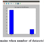
The table indicates the performance testing of three methods gives the GM1 has 85% land region than IMM product and 14.9% of sea region whereas the APM and IMM products has land ranging from 77-84% and sea 16-23 %.
Table 7: 50 datasets as input and each dataset produces 20 smaller divided blocks.
| S. No |
Product Domain |
Product/Dataset Number |
No. of blocks |
| 1 |
ASA_AMP |
50 |
50*20=1000 |
| 2 |
ASA_IMM |
50 |
1000 |
| 3 |
ASA_GMM |
50 |
1000 |
Table 8: The land and sea percentages of the surface area detected for three domains
| Domain/Product |
Number of blocks |
Land Percentage |
Sea percentage |
| ASA_APM |
1000 |
83.371032 |
16.628968 |
| ASA_IMM |
1000 |
77.675842 |
22.324158 |
| ASA_GM1 |
1000 |
85.047632 |
14.952368 |
Global Monitoring Mode (GM1) is increasing the number of partitioning chunks which gives more land region and less sea region. Whereas the APM product retains the stable percentage of land as well as the sea regions and it producing large of dissimilarity among percentages of regions is not seen in performance testing.
In the case of Image Mode Medium Resolution Image (IMM) the land percentages are decreasing as increasing the number of chunks. The number of images in the area of IMM is utilized for performance testing gives a slow decrease in land and sea regions.
Conclusions
In our proposed method, the overall result by analyzing the dissimilar domains in the remote sensing satellites which is uninterruptedly releasing the data. With different types of products are increasing we observed and analyzed the data behave with regard to land and sea surface regions. The data from satellite emitting continuously, surface area analysis will be less in time when different areas by diverse products are in use and analyze the surface regions. For analysis of a large number of surface regions required high Processing computational devices for ex, if we take 10 surface regions will require more than 500 products for each domain.
Future Work
In further, we will extend our proposed method not only for calculated and categorize the land and sea regions but also include diverse areas like forest areas, sand areas etc. we extending this work for predicting the earthquakes, tsunamis and natural disasters that can be recognized with analysis of proper recommendation to avoid the natural disasters. In future, we analyze rainfall prediction by utilizing the parameters like Co2, hydrogen, nitrogen contents in the air and corresponding land area whether the chance of rainfall is there or not.
References
- http://www.colorado.edu/geography/gcraft/notes/remote/remote_f.html
- https://prezi.com/i1hrip789ruy/orbits-and-satellites.
- http://www.oneonta.edu/faculty/baumanpr/geosat2/RS%20History%20II/RS-History-Part-2.html
- Harshaverdana et al., “Aadoption of Hadoop for a remote sensing real time big data analysis” international Journal of Advance Research in Engineering, Science &Technology,June-2016; Volume 3, Issue 6: e-ISSN: 2393 -9877, p- ISSN: 2394-2444.
- J. Shi, et al., “Change detection in synthetic aperture radar image based on fuzzy active contour”Mathematical Problems in Engineering Volume 2014 (2014), Article ID 870936, http://dx.doi.org/10.1155/2014/870936.
CrossRef
- Sheik Mujabar et al., Coastal erosion hazard and vulnerability assessment for southern coastal Tamil Nadu of India by using remote sensing and GIS. Nat Hazards. (2013); 69(3):1295–314.
- Chu ZX et al., Changing pattern of accretion/erosion of the modern Yellow River (Huanghe) subaerial delta, China: Based on remote sensing images. Mar Geol. (2006); 227(1–2):13–30.
- Cowart L., et al., Shoreline change along sheltered coastlines: Insights from the neuse river estuary, NC, USA. Remote Sens. (2011); 3(7):1516–34.
- RUHOFF, A. L., et al., Modelagem ambiental com a simulação de cenários preservacionistas. 93 f. Dissertação (Mestrado em Geomática) – Universidade Federal de Santa Maria, Santa Maria, 2004.

This work is licensed under a Creative Commons Attribution 4.0 International License.