Introduction
The Internet of Things (IoT) might be thought of as the
designation of Ubiquitous Computing. In IoT, the user environment is replete of
gadgets working cooperatively.1, 2, 3 These gadgets go from
computing elements, for example, RFID tags and biochip on ranch animals to
smartphones and machines with implicit sensors. Types of gear like these are
known by the name of “things”. In any case, programming these frameworks
is additionally challenging, due, not only to their sheer volume but also to
their diversity.4 Botnet attacks have destroyed the effect on public
and private frameworks. The botmasters controlling these systems mean to
counteract bring down endeavors by utilizing very versatile peer to peer
overlays to lay hold of their botnets, and even solidify them with
countermeasures against intelligence gathering endeavors. Ongoing research
demonstrates that advanced countermeasures can hamper the capacity to accumulate
the fundamental intelligence for bringing down botnets.5
On the other hand, adapting to malware is getting
increasingly challenging, given their constant development in intricacy and
volume. A standout amongst the most widely recognized methodologies in writing
is utilizing machine learning methods, to simply learn models and patterns
behind such intricacy, and to create methods to keep pace with malware
development.6 Supervised Learning is one of the methods under
Machine learning that it is on the application layer. Application layer and
protocol layer are two layers under passive monitoring which is one of the
methods under Network based on Anomaly-based that it is part of Intrusion
Detection System classification (IDS). The Supervised Learning techniques also
called the Classification methods is a type of technique that includes the
target and dependent variable that is to be forecasted from a given set of
independent variables. Therefore, it can produce the function that maps inputs
to needed outputs using those sets of variables (training data). The training
process will be continued until the model reaches the desired level of accuracy
on training data.7 According to our previous study, it reviewed some recent
studies that have been done on a Machine learning algorithm to identify Botnet.
On supervised learning methods, the statistical foundation like hypothesis
representation, concerns about the relationship between the features “x” and
target “y”. That should be defined via the selected features as well as accepts
some ample information regarding what that action is similar in the way to
perfectly demonstrate the activities of bots using supervised learning methods.
Detecting bots based on certain well-known and particular features have been
used in supervised learning methods. The accuracy of supervised learning
methods could be effective against bot traffic which seeks for covering up
itself between legitimate traffic by given certain particular malicious traffic
features. However, most of the supervised learning methods have a common trend
also separately from particular perceptions toward traffic of bot shown in the
feature space, supervised learning techniques accomplish poorly. Supervised
learning techniques might overcome the secret nature of bots. Supervised
learning techniques are worked for cases that certain particular characteristic
is known.7
This research will study the several Supervised Learning
methods which are; Linear Regression, Logistic Regression, Decision Tree, Naive
Bayes, k- Nearest Neighbors, Random Forest, Gradient Boosting Machines, and
Support Vector Machine for identifying the Botnet in IoT. This study aims to
find which Supervised Learning technique can achieve the highest accuracy and
fastest detection as well as with minimizing the dependent variable.
Data sources and
Instrumentation
To evaluate the classification performance of bots and
botnet domain names using machine learning techniques, the extracted labeled
domain name datasets that include the set of normal domain names and malicious
domain names that have been used via Botnets will be used in this research. The
set of normal domains name includes 790,745 domain names. Normal domain names
will be checked at www.virustotal.com to verify that they are a normal domain.
On the other hand, the set of malicious domain names (total number of 199,772)
collected from three different sources which are: 1- www.cert.at 2-
www.github.com and 3- www.kaggle.com. All domain names including the normal and
malicious domain names have 204 variables such as the IP address, port number,
SRC port, DST port, packet pay size, idle time max, HTTP response status code,
packet header size, payload bytes max, HTTP request version, packets ack avg,
packet direction, and so on. This research will firstly select five training
datasets randomly which include both normal domain names and malicious domain
names from data sources mentioned above. After that, one testing datasets which
include both normal and malicious domain names from data sources but not from
those which was selected for training datasets will be selected. In this study,
a few classification measures such as False Positive (FP), True Positive (TP),
False Negative (FN), True Negative (TN), and accuracy (ACC) will be used. After
that will be used the suggested Supervised Learning algorithms on those
training datasets and testing dataset to identify the best one in terms of
accuracy and performance.
Implementation
After setting up the training dataset and testing dataset we
have done analyzing individual feature statistics of variables and finding the
correlation and apparent relationships between the variables to minimizing the
number of variables that needed for identifying the Botnet without reducing the
accuracy as well as avoiding increasing the duration of detection. We narrow it
down from 204 variables to only 20 variables. Then we examine it on selected
Supervised Learning methods to find out which one has the highest accuracy with
the lowest time duration.
Linear Regression
One of the oldest and most widely used analytics methods is
the technique of regression. The objective of regression is to deliver a model
that represents the ‘best fit’ to some observed data. Commonly the model is a
capacity depicting some kind of bend (lines, parabolas, and so on.) that is
dictated by a lot of parameters (e.g., slope and intercept). “Best
fit” implies that there is an ideal arrangement of parameters as indicated
by an evaluation criterion we pick. A regression model endeavors to foresee the
estimation of one variable, known as the dependent variable, response variable
or label, utilizing the values of different variables, known as independent
variables, explanatory variables or features. Single regression has one label
used to foresee one feature. Multiple regression utilizes at least two feature
variables.8
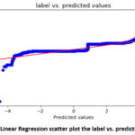
Based on the apparent
relationships identified when analyzing the data, a linear regression model was
created to predict the value for the label (either they are normal domain names
or malicious domain names), from which the predicted label can be calculated.
The model was trained with 80% of the data and tested with the remaining 20%.
The Root Mean Square Error (RMSE) for the test results is 0.3878 and the
standard deviation of the label is 0.1066. Also, to make all features
standardization, we used the standard scaler to do standard normally
distributed data. Since the model predicts log of the label, the results are is
in float not in integer and due to the domain names are either normal domain
(0) or malicious domain (1). To make it more accurate we round the predicted
values to an integer. Indicating that there is a model performs reasonably
well. The predicted label is converted back to its exponential value (the
rounded label), which leads to fit well with The RMSE of 0.4378 and a standard
deviation of 0.1270 and an accuracy of 0.8090 (80.90%). The True Positive (TP)
1.30%, True Negative (TN) 79.60%, False Positive (FP) 0.21 %, and False
Negative (FN) 18.89% is after rounding the results which mean achievement of
80.90%. A scatter plot showing the predicted log label and the actual log label
is shown in Figure 1.
Logistic Regression
Logistic Regression is a classification, not a regression
algorithm. It is utilized to evaluate discrete values (Binary values like 0/1,
yes/no, true/false) dependent on a given arrangement of the independent
variable(s). In straightforward words, it predicts the likelihood of an event
of an occasion by fitting information to a logit function. Thus, it is
otherwise called logit relapse. Since it predicts the likelihood, its yield
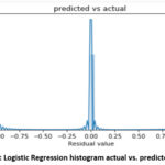
esteems lies somewhere in the range of 0 and 1.9 Based on the
apparent relationships identified when analyzing the data, the Logistic
Regression model was created to predict the value for the label (either they
are normal domain names or malicious domain names), from which the predicted
label can be calculated. The model was trained with 80% of the data and tested
with the remaining 20%. The RMSE for the test results is 0.4271 and the
standard deviation of the label is 0. Also, to make all features
standardization, we used the standard scaler to do standard normally
distributed data, indicating that there is a model that performs reasonably
well and also the accuracy of 0.8175 (81.75%). The True Positive (TP) 4.64%,
True Negative (TN) 77.11%, False Positive (FP) 2.66%, and False Negative (FN) 15.59%
are the results which mean achievement of 81.75% or on the other hand 18.25%
detecting wrongly. A histogram plot showing the predicted log label and the
actual log label is shown in Figure 2.
Decision Tree
Decision Tree is a sort of supervised learning calculation
that is for the most part utilized for classification issues. Incredibly, it
works for both categorical and continuous dependent variables. A decision tree
is a choice help device that utilizes a tree-like model of choices and their
conceivable results, including chance occasion results, asset expenses, and
utility. It is one approach to show a calculation that just contains
restrictive control explanations. Decision trees are generally utilized in
operations research, explicitly in a choice examination, to help recognize a
methodology well on the way to achieve an objective, but on the other hand, are
a popular tool in machine learning.10
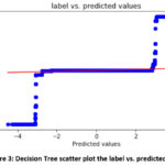
Based on the apparent relationships identified when
analyzing the data, a Decision Tree model was created to predict the value for
the label (either they are normal domain names or malicious domain names), from
which the predicted label can be calculated. The model was trained with 80% of
the data and tested with the remaining 20%. The RMSE for the test results is
0.0477 and the standard deviation of the label is 0.4010. Also, to make all
features standardization, we used the standard scaler to do standard normally
distributed data. Indicating that there is a model performs reasonably well.
The result leads to fit well with the accuracy of 0.9976 (99.76%). The True
Positive (TP) 20.99%, True Negative (TN) 78.77%, False Positive (FP) 0.11%, and
False Negative (FN) 0.13% is after rounding the results which mean achievement
of 99.76% or on the other hand 0.24% detecting wrongly. A scatter plot showing
the predicted log label and the actual log label is shown in Figure 3.
Naive Bayes
Naive Bayes is a classification method dependent on Bayes’
hypothesis with an assumption of independence between predictors. In basic
terms, a Naive Bayes classifier expects that the nearness of a specific feature
in a class is unrelated to the nearness of some other element. For instance, a
fruit might be viewed as an apple in the event that it is red, round, and
around 3 inches in distance across. Regardless of whether these highlights rely
upon one another or upon the presence of alternate highlights, a naive Bayes
classifier would consider these properties to independently add to the
likelihood that this fruit product is an apple. Naive Bayes model is anything
but difficult to construct and especially useful for very large data sets.
Alongside effortlessness, Naive Bayes is known to outperform even highly
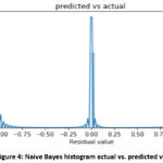
sophisticated classification methods.11 Based on the apparent
relationships identified when analyzing the data, the Naive Bayes model was
created to predict the log-normal value for the label (either they are normal
domain names or malicious domain names), from which the predicted label can be
calculated. The model was trained with 80% of the data and tested with the
remaining 20%. The RMSE for the test results is 0.4626 and the standard
deviation of the label is 0.0. Also to make all features standardization, we
used the standard scaler to do standard normally distributed data, indicating
that there is a model performs reasonably well and also the accuracy of 0.7859
(78.59%). The True Positive (TP) 1.65%, True Negative (TN) 76.94%, False
Positive (FP) 2.84%, and False Negative (FN) 18.57% are the results which mean
achievement of 78.59% or on the other hand 21.41% detecting wrongly. A histogram
plot showing the predicted log label and the actual log label is shown in
Figure 4.
k- Nearest Neighbors
k- Nearest Neighbors (k-NN) can be utilized for both
classification and regression issues. Nonetheless, it is all the more generally
utilized classification problems in the business. K nearest neighbors is a
straightforward algorithm that stores every available case and classifies new
cases by a majority vote of its k neighbors. The case being doled out to the
class is most common among its K nearest neighbors estimated by a distance
function. k-NN calculation is a non-parametric technique utilized for classification
and regression. In the two cases, the information comprises of the k nearest
preparing models in the feature space. The output relies upon whether k-NN is
utilized for classification or regression. In k-NN classification, the yield is
class participation. An item is classified by a majority vote of its neighbors,
with the object being given to the class most basic among its k closest
neighbors (k is a positive integer, normally small). If k = 1, at that point
the item is essentially allocated to the class of that single nearest neighbor.
In k-NN regression, the output is the property estimation for the object. This
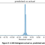
value is the average of its k nearest neighbors.12 Based on the
apparent relationships identified when analyzing the data, the k- Nearest
Neighbors model was created to predict the log-normal value for the label
(either they are normal domain names or malicious domain names), from which the
predicted label can be calculated. The model was trained with 80% of the data
and tested with the remaining 20%. The RMSE for the test results is 0.1093 and
the standard deviation of the label is 0.0. Also to make all features
standardization, we used the standard scaler to do standard normally
distributed data, indicating that there is a model that performs reasonably
well and also the accuracy of 0.9880 (98.80%). The True Positive (TP) 19.22%,
True Negative (TN) 79.58%, False Positive (FP) 0.20%, and False Negative (FN)
1% are the results which mean achievement of 98.80% or on the other hand 1.20%
detecting wrongly. A histogram plot showing the predicted log label and the
actual log label is shown in Figure 5.
Random Forest
Random forest or random decision forest is a group learning
strategy for classification, regression and different undertakings that works
by building a large number of decision trees at training time and yielding the
class that is the method of the classes (classification) or mean prediction
(regression) of the individual trees. Random choice forests correct for
decision trees’ practice for overfitting to their training set. Random Forest
is a trademarked term for a group of decision trees. In Random Forest, we have
an accumulation of decision trees (so-known as “Forest”). To order
another item dependent on characteristics, each tree gives a classification and
we state the tree “votes” for that class. The forest picks the
classification having the most votes (over every one of the trees in the
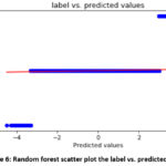
forest).13 Based on the apparent relationships identified when
analyzing the data, a random forest model was created to predict the log-normal
value for the label (either they are normal domain names or malicious domain
names), from which the predicted label can be calculated. The model was trained
with 80% of the data and tested with the remaining 20%. The RMSE for the test
results is 0.0422 and the standard deviation of the label is 0.0. Also to make
all features standardization, we used the standard scaler to do standard
normally distributed data. Indicating that there is a model performs reasonably
well. The result leads to fit 100% with an accuracy of 0.9982 (99.82%). The
True Positive (TP) 20.09%, True Negative (TN) 79.73%, False Positive (FP)
0.04%, and False Negative (FN) 0.14% is after rounding the results which mean
achievement of 99.82% or on the other hand 0.18% detecting wrongly. A scatter
plot showing the predicted log label and the actual log label is shown in
Figure 6.
Gradient Boosting
Machines (GBM)
GBM is a machine learning method for classification and
regression issues, which creates an expectation model in the form of an
ensemble of weak forecast models, commonly decision trees. It assembles the
model in a phase shrewd style as other boosting strategies do, and it sums them
up by permitting advancement of a subjective recognizable detriment function.
Gradient Boosting Machines is a boosting calculation utilized when we manage a
lot of information to make a forecast with high expectation control. Boosting
is a gathering of learning calculations which consolidates the forecast of a
few base estimators to improve power over a single estimator. It joins numerous
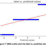
feeble or normal indicators to build a strong predictor.14 Based on
the apparent relationships identified when analyzing the data, a Gradient
Boosting Machines model was created to predict the log-normal value for the
label (either they are normal domain names or malicious domain names), from
which the predicted label can be calculated. The model was trained with 80% of
the data and tested with the remaining 20%. The RMSE for the test results is
0.2033 and the standard deviation of the label is 0.0. Also, to make all
features standardization, we used the standard scaler to do standard normally
distributed data. Indicating that there is a model performs reasonably well.
The result leads to fit well with an accuracy of 0.9586 (95.86%). The True
Positive (TP) 17.03%, True Negative (TN) 78.83%, False Positive (FP) 0.95%, and
False Negative (FN) 3.19% is after rounding the results which mean achievement
of 95.86% or on the other hand 4.14% detecting wrongly. A scatter plot showing
the predicted log label and the actual log label is shown in Figure 7.F
Table 1: The summary
results of each supervised learning algorithm.
| Algorithm | TP | TN | FP | FN | ACC |
| Linear Regression |
1.30%
|
79.60%
|
0.21%
|
18.89%
|
80.90%
|
| Logistic Regression |
4.64%
|
77.11%
|
2.66%
|
15.59%
|
81.75%
|
| Decision Tree |
20.99%
|
78.77%
|
0.11%
|
0.13%
|
99.76%
|
| Naive Bayes |
1.65%
|
76.94%
|
2.84%
|
18.57%
|
78.59%
|
| k-NN |
19.22%
|
79.58%
|
0.20%
|
1%
|
98.80%
|
| Random Forest |
20.09%
|
79.73%
|
0.04%
|
0.14%
|
99.82%
|
| GBM |
17.03%
|
78.83%
|
0.95%
|
3.19%
|
95.86%
|
| SVM |
Out of Time
|
Out of Time
|
Out of Time
|
Out of Time
|
Out of Time
|
Support Vector Machine (SVM)
Support Vector Machines (SVM) are supervised learning models
with associated learning algorithms that analyze data used for classification
and regression analysis. Given a set of training examples, each marked as
belonging to one or the other of two categories, a SVM training algorithm
builds a model that assigns new examples to one category or the other, making
it a non-probabilistic binary linear classifier (although methods such as Platt
scaling exist to use SVM in a probabilistic classification setting). A Support
Vector Machines display is a portrayal of the precedents as focuses in space,
mapped with the goal that the instances of the different classes are separated
by a reasonable hole that is as wide as could be expected under the
circumstances. New precedents are then mapped into that equivalent space and
anticipated to have a place with a class dependent on which side of the hole
they fall.15 Based on the apparent relationships identified when analyzing the
data, the SVM model was created to predict the log-normal value for the label
(either they are normal
domain names or malicious domain names), from which the
predicted label can be calculated. The model was trained with 80% of the data
and tested with the remaining 20%. However, we run for one week but the
processing was not done therefore we reduced the training data to 10% and also
used Dimensionality Reduction Algorithm (PCA) to reduce the number of random
variables under consideration by obtaining a set of principal variables.
Nevertheless, after done all still could not get the results in a reasonable time.
Conclusion
This study examines the Supervised Learning algorithms for
identifying the Botnets and bots in the Internet of Things network. Which the
summary of the results can be found in table 1. From eight supervised learning
techniques only 4 of them could achieve above 90% accuracy which is: 1- k-
Nearest Neighbors: although it achieves 98.80% accuracy the duration taken from
run the code to get the result was 118 seconds and 94 milliseconds, 2- Decision
Tree: it achieves 99.76% accuracy with the duration taken from run the code to
get the result was 31 seconds and 10 milliseconds, 3- Random Forest: although
it achieves 99.82% accuracy but the duration is taken from run the code to get
the result was 84 seconds and 72 milliseconds, and 4- Gradient Boosting
Machines: although it achieves 95.86% accuracy the duration is taken from run
the code to get the result was 164 seconds and 81 milliseconds.
With the consideration from the above data collected from
this research, even though the Random Forest has the highest accuracy rate
(99.89%) but the duration taken from run the code to get the result was high
(84 seconds and 72 milliseconds) while the Decision Tree has done in just 31
seconds and 10 milliseconds with only 0.06% lower accuracy than the Random
Forest and since the speed of detecting is one of this research aim, the
Decision Tree is the best to identifying the Botnets and bots in the Internet
of Things with high accuracy (99.76%) on lowest time duration from run the code
to get the result among of supervised learning methods which studied in this
research.
Aknowledgements
As corresponding author I, Amirhossein Rezaei, hereby
confirm on behalf of all authors that:
- This manuscript, or a large part of it, has not
been published, to any other journal.
- All text and graphics, except for those marked
with sources, are original works of the authors, and all necessary permissions
for publication were secured prior to submission of the manuscript.
- All authors each made a significant contribution
to the research reported and have read and approved the submitted manuscript.
Conflict of Interest
We wish to draw the attention of the Editor to the following
facts which may be considered as potential conflicts of interest and to
significant financial contributions to this work. [OR] We wish to confirm that
there are no known conflicts of interest associated with this publication and
there has been no significant financial support for this work that could have
influenced its outcome.
We confirm that the manuscript has been read and approved by
all named authors and that there are no other persons who satisfied the
criteria for authorship but are not listed. We further confirm that the order
of authors listed in the manuscript has been approved by all of us.
We confirm that we have given due consideration to the
protection of intellectual property associated with this work and that there
are no impediments to publication, including the timing of publication, with
respect to intellectual property. In so doing we confirm that we have followed
the regulations of our institutions concerning intellectual property.
We understand that the Corresponding Author is the sole
contact for the Editorial process (including Editorial Manager and direct
communications with the office). He/she is responsible for communicating with
the other authors about progress, submissions of revisions and final approval
of proofs. We confirm that we have provided a current, correct email address
which is accessible by the Corresponding Author and which has been configured
to accept email from (ahr338@gmail.com).
References
- Jayavardhana Gubbi, Rajkumar Buyya, Slaven Marusic, Marimuthu Palaniswami, Internet of Things (IoT): A vision, architectural elements, and future directions, ELSEVIER, Future Generation Computer Systems, Volume 29, Issue 7, Pages 1645-1660, Sep 2013.
CrossRef - Eleonora Borgia, The Internet of Things vision: Key features, applications and open issues, ELSEVIER, Computer Communications, Volume 54, Pages 1-31, 1 Dec 2014.
CrossRef - Luigi Atzori, Antonio Iera, Giacomo Morabito, The Internet of Things: A survey, ELSEVIER, Computer Networks, Volume 54, Issue 15, Pages 2787-2805, 28 Oct 2010.
CrossRef - Fernando A.Teixeira, Fernando M.Q.Pereira, Hao-Chi Wong, José M.S.Nogueira, Leonardo B.Oliveira, SIoT: Securing Internet of Things through distributed systems analysis, ELSEVIER, Future Generation Computer Systems, Volume 92, Pages 1172-1186, March 2019.
CrossRef - Leon Böck, Emmanouil Vasilomanolakis, Jan Helge Wolf, Max Mühlhäuser, Autonomously detecting sensors in fully distributed botnets, ELSEVIER, Computers & Security, Volume 83, Pages 1-13, June 2019.
CrossRef - Daniele Ucci, Leonardo Aniello, Roberto Baldoni, Survey of machine learning techniques for malware analysis, ELSEVIER, Computers & Security, Volume 81, Pages 123-147, March 2019.
CrossRef - Amirhossein Rezaei, Identifying Botnet on IoT and Cloud by Using Machine Learning Techniques, Open International Journal of Informatics (OIJI), 2018.
- Matias D. Cattaneo, Michael Jansson, Whitney K. Newey (2018). Inference in Linear Regression Models with Many Covariates and Heteroscedasticity. Journal of the American Statistical Association.Volume 113, 2018 – Issue 523.
CrossRef - Taedong Kim and Stephen J. Wright (2018). PMU Placement for Line Outage Identification via Multinomial Logistic Regression. IEEE Transactions on Smart Grid. Volume. 9 , Issue. 1.
CrossRef - Raza Hasan, Sellappan Palaniappan, Abdul Rafiez Abdul Raziff, Salman Mahmood, Kamal Uddin Sarker (2018). Student Academic Performance Prediction by using Decision Tree Algorithm. 4th International Conference on Computer and Information Sciences (ICCOINS).
CrossRef - Tong Li, Jin Li, Zheli Liu, Ping Li, Chunfu Jia (2018). Differentially private Naive Bayes learning over multiple data sources. Elsevier, Information Sciences, Volume 444, May 2018, Pages 89-104.
CrossRef - Xueyan Wu, Jiquan Yang, Shuihua Wang (2018). Tea category identification based on optimal wavelet entropy and weighted k-Nearest Neighbors algorithm. Springer Science+Business Media New York.
CrossRef - Jaime Lynn Speiser, Bethany J.Wolf, Dongjun Chung, Constantine J.Karvellas, David G.Koch, Valerie L.Durkalski (2019). BiMM forest: A random forest method for modeling clustered and longitudinal binary outcomes. Elsevier, Chemometrics and Intelligent Laboratory Systems, Volume 185, 15 February 2019, Pages 122-134.
CrossRef - Xing Chen, Li Huang, Di Xie, Qi Zhao (2018). EGBMMDA: Extreme Gradient Boosting Machine for MiRNA-Disease Association prediction. Cell Death & Diseasevolume 9, Article number: 3 (2018).
CrossRef - Jakob Ziegier, Hubert Gattringer, Andreas Mueller (2018). Classification of Gait Phases Based on Bilateral EMG Data Using Support Vector Machines. 2018 7th IEEE International Conference on Biomedical Robotics and Biomechatronics (Biorob).
CrossRef

This work is licensed under a Creative Commons Attribution 4.0 International License.