Introduction
Textures are complex visual patterns composed of entities, or sub patterns that have characteristic brightness, color, slope, size. Thus texture can be regarded as a similarity grouping in an image (Rosenfeld 1982). The local sub-pattern properties give rise to the perceived lightness, uniformity, density, roughness, regularity, linearity, frequency, phase, directionality, coarseness, randomness, fineness, smoothness, granulation of the texture as a whole (Levine 1985).
Types of Iris Textures
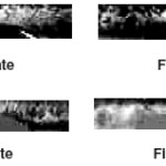
The texture of the iris is determined by the arrangement of the white fibers radiating from the center of the iris. All iris contain these fibers but in some it is a challenge to discern them. Depending on the texture, we can group the human iris into four basic groups. They are Stream iris, Jewel iris, Shaker iris and Flower iris respectively [1]. Also, there are different combinations of these groups. The proposed work mainly concentrates on grouping the given database into the above four classes.
Stream Iris
It contains a uniform fiber structure with subtle variations or streaks of color as shown in Figure 1.1.a. The structure of the iris is determined by the arrangement of the white fibers radiating from the center of the iris (or pupil). The fibers are roughly parallel, evenly arranged and vary only in density and intensity. In thisimage one can notice that they are uniform and reasonably direct or parallel.
Jewel Iris
It contains dot like pigments in the iris. The jewel iris can be recognized by the presence of pigmentation or colored dots on top of the fibers as shown in Figure 1.1.b. The dots (or jewels) can vary in color from light orange through black. They can also vary in size from tiny (invisible to the naked eye) to quite large. The pigmentation is superimposed above the fibers. This usually is much easier to identify than a Stream iris; but if an iris looks to be 90% Stream and 10% Jewel, it would be treated as a jewel.
Shaker iris
It contains dot-like pigments and rounded openings. The shaker iris is identified by the presence of both flowers like petals in the fiber arrangement and pigment dots or jewels as shown in Figure 1.1.d.The presence of both flower and jewel characteristics is the key to the Shaker iris structure. The presence of even one jewel in an otherwise Flower iris is sufficient to cause the occupant to exhibit Shaker characteristics.
Flower iris
It contains distinctly curved or rounded openings in the iris. In a flower iris the fibers radiating from the center are distorted (in one or more places) to produce the effect of petals (hence the name flower) shown in Figure 1.1.c. In this image one can notice that they are neither regular nor uniform. A flower iris may have only one significant petal with the remainder of the iris looking like a stream. The fibers form rounded openings in the iris; these vary in size, density and intensity and are likely to be more apparent in the left eye.
Fractal-based metrics capture texture properties, such as the ranges and frequency of self-similar surface peaks, which is not possible with traditional measures2. Fractal dimension extracts roughness information from images considering all available scales at once3. Single scale features may not be sufficient to characterize the textures, thus multiple scale features are considered necessary for a more complete textural representation4.
Wavelets are employed for the computation of single and multiple scale roughness features due to their ability to extract information at different resolutions.
Recent developments involve decomposition of the image in terms of wavelets which provide information about the image contained in smaller regions also. Gabor filters5 and Haar wavelets6 can be used for this purpose. A Wavelet transformation converts data from the spatial into the frequency domain and then stores each component with a corresponding matching resolution scale6. Wavelets are used to represent different levels of details. The Haar wavelet is one of the simplest wavelet transforms used to decompose the image into different frequency sub-bands. Using all frequency bands for classification may increase the time complexity of algorithms. Thus only significant sub-bands are selected for classification based on energy and entropy7. Also selecting weak sub-bands may affect performance of classification algorithms.
In this work, a novel approach unifying the advantages of both fractal dimensions and wavelet sub-bands is proposed for iris texture classification. Fractal dimension such as Minkowski dimension is used to decompose the sub-bands at each level in tree structure of Haar wavelet decomposition. Further various statistical features of these significant sub-bands are used to construct the feature vector. Modified K-NN classifier is used to recognize the texture. Both probabilistic and non probabilistic classifiers such as Euclidean, Bayes and conventional K-NN are used for comparative study. The rest of the paper is organized as follows: Section 2 introduces the proposed method and also describes the implementation details. Section 3 comes out with experimental results and their discussion and section 4 concludes the whole paper.
Proposed Method
The process of iris texture classification typically involves the following stages: (a) estimation of fractal dimension of each resized iris template
decomposition oftemplate into significant sub-bands using 5 level Haar wavelet based on fractal dimension (c) extraction of feature vector using statistical features of sub-bands (d) Classifications, both probabilistic andnon probabilistic classifiers such as Bayes, Euclideanand K-Nearest Neighbor are used for classification of iris templates.
Fractal dimension
The word fractal refers to the degree of self similarity at different scales. Fractal dimension can be used to discriminate between textures of similar sets. Box counting method is one of the wide varieties of methods for estimating the fractal dimension8, which can be automatically applied to patterns with or without self similarity. This FD can be also called as entropy dimension, Kolmogorov entropy, capacity dimension, metric dimension and Minkowski dimension. It provides description of how much of the surface it fills.
An image of size R x R pixels, is partitioned into grids measuring s x s, where 1 ≤ s ≤ R/2. Then r = s/R. If the minimum and maximum gray scale levels in the (i, j)th grid fall into the kth and lth boxes, respectively the contributions of nr in the (i, j)th grid is defined as

Nr is computed from different values of r and the fractal dimension FD can be estimated as the slope of the line joining these points (log (1/r), log Nr). The linear regression equation to estimate the fractal dimension is

where k is a constant and FD denotes dimension of the fractal set.
Decomposition
Haar transform is real and orthogonal. Haar Transform is a very fast transform. The basis vectors of the Haar matrix are sequence ordered. The original signal is split into a low and a high frequency parts and then filters will do the splitting without duplicating information and they may be called orthogonal. The magnitude response of the filter is exactly zero outside the frequency range covered by the transform. If this property is satisfied, the transform is energy invariant.
Table 1: Fractal dimensions of Bark texture image sub-bands
|
Resolution
|
Sub-bands
|
|
|
WLL
|
WHL
|
WLH
|
WHH
|
|
Level 1
|
2.2247
|
2.1954
|
2.2125
|
2.1962
|
|
Level 2
|
2.1819
|
2.1925
|
2.2027
|
2.1605
|
|
Level 3
|
2.2063
|
2.1749
|
2.1968
|
2.1566
|
|
Level 4
|
2.1772
|
2.2030
|
2.1997
|
2.1757
|
|
Level 5
|
2.1875
|
2.1687
|
2.1654
|
2.1600
|
|
Level 6
|
2.1472
|
2.1575
|
2.1769
|
2.1456
|
|
Level 7
|
2.1734
|
2.1667
|
2.1768
|
2.1498
|
|
Level 8
|
2.1642
|
2.1477
|
2.1596
|
2.1406
|
Table 2: Feature vectors for classification of Bark texture image
|
Resolution(i)
|
Sub band Selected
|
F1 iBrightness
|
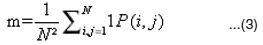
(m)
|
F2 iContrast(Sd)
|
F3 iEnergy(E)
|
|
Level 1
|
LL
|
0.6674
|
|
0.2311
|
3.2691e+004
|
|
Level 2
|
LH
|
0.2274
|
|
0.1463
|
4.7938e+003
|
|
Level 3
|
LL
|
0.4279
|
|
0.1375
|
1.3238e+004
|
|
Level 4
|
HL
|
0.2626
|
|
0.1411
|
5.8255e+003
|
|
Level 5
|
LL
|
0.4692
|
|
0.1224
|
1.5409e+004
|
|
Level 6
|
LH
|
0.2678
|
|
0.1380
|
5.9482e+003
|
|
Level 7
|
LH
|
0.2570
|
|
0.1565
|
5.9340e+003
|
|
Level 8
|
LL
|
0.4639
|
|
0.1439
|
1.5460e+004
|
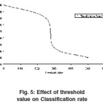
Table 3: Effect of threshold value on classification rate of Bark texture
|
Threshold value(λ)
|
Number of levels decomposed
|
Classification Rate %
|
|
0.00
|
8
|
100
|
|
0.025
|
6
|
96
|
|
0.03
|
2
|
87
|
|
0.05
|
1
|
84
|
Table 4: Significant co-occurrence features of original images of different textures
|
|
F1
|
F2
|
F3
|
F4
|
F5
|
F6
|
|
Bark
|
-2.1214e+012
|
4.5655e+011
|
2.4350e+012
|
9.8300e+006
|
-8.8347e+040
|
6.1037e+051
|
|
Grass
|
-2.1210e+012
|
3.9936e+011
|
3.6371e+012
|
9.6927e+006
|
-8.9721e+040
|
6.2306e+051
|
|
Leather
|
-2.1214e+012
|
3.5028e+011
|
5.3788e+012
|
1.0630e+007
|
-8.8097e+040
|
6.0807e+051
|
|
Wood
|
-2.0980e+012
|
1.9805e+011
|
1.7729e+013
|
1.5164e+007
|
-2.1135e+041
|
1.9529e+052
|
|
Sand
|
-2.1081e+012
|
1.6377e+011
|
1.4469e+013
|
1.6176e+007
|
-1.4970e+041
|
1.2330e+052
|
|
Straw
|
-2.1078e+012
|
2.4294e+011
|
7.5384e+012
|
1.2623e+007
|
-1.5149e+041
|
1.2527e+052
|
|
Weave
|
-2.1201e+012
|
7.7293e+011
|
1.8764e+012
|
7.6606e+006
|
-9.3480e+040
|
6.5811e+051
|
|
Woolen
|
-2.1130e+012
|
1.6206e+011
|
1.2738e+013
|
1.5278e+007
|
-1.2458e+041
|
9.6514e+051
|
|
Water
|
-2.1030e+012
|
1.6104e+011
|
1.4238e+013
|
1.6018e+007
|
-1.3958e+041
|
1.6514e+051
|
F1: Cluster Tendency, F2:Contrast, F3: Energy, F4:Local Homogeneity,F5:Cluster Shade, F6: Cluster Prominence
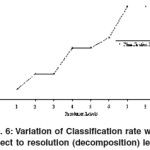
Table 5: Effect of resolution on classification rate (Bark texture)
|
Resolution
|
Classification rate %
|
|
Level 1
|
84
|
|
Level 2
|
87
|
|
Level 3
|
87
|
|
Level 4
|
92
|
|
Level 5
|
92
|
|
Level 6
|
94
|
|
Level 7
|
100
|
|
Level 8
|
100
|
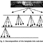
In the Haar transform, it has the perfect reconstruction property since the input signal is transformed and inversely transformed by using a set of weighted basis functions and the reproduced sample values are identical to those of the input signal. Also it is ortho-normal since no information redundancy is present in the sampled signal. The Haar wavelet transform has a number of advantages like simplicity, fastness, memory efficiency and reversibility when compared with other wavelets. A 8-level Haar wavelet is decomposed into LL1, LL8, HL1 to HL8 (horizontal coefficients), LH1 to LH8 (vertical coefficients) and HH1 to HH8 (diagonal coefficients). Among these only some of the sub-bands have significant energy and entropy of the texture patterns. Such sub-bands are decomposed in the next level.
Sub band Selection and Feature Extraction
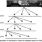
Fractal dimension values for each sub band at each decomposition level are estimated. The sub band that has highest FD value is chosen for decomposition into next level and so on. In order to save processing time the decomposition must be terminated somewhere. This may be done when there is no significant difference between the FD values. This can be achieved by introducing some threshold value λ, such that the absolute difference Df = |f1j-f2j| between all four wavelets sub-bands for a certain decomposition level is less than or equal to that value13.
As we have selected the significant sub-bands based on FD there is no need to measure for the second time. FD used in this work is based on the entropy of the image. Remaining features such as contrast, brightness and energy of significant sub-bands of five levels decomposed images are calculated as features and feature vector is formed with these values.
Mean(m) represents average brightness of the sub-band
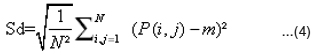
Standard Deviation (sd) represents contrast of the sub band
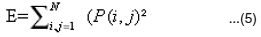
Energy of sub band is given by
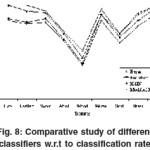
Table 6: Comparative study of modified K-NN with other classifiers
|
Texture
|
Classification Rate %
|
|
|
Bayes
|
Euclidean
|
K-NN
|
Modified K-NN
|
|
Bark
|
84
|
86
|
100
|
100
|
|
Leather
|
80
|
82
|
94
|
100
|
|
Water
|
82
|
86
|
92
|
94
|
|
Wool
|
62
|
64
|
70
|
72
|
|
Wood
|
36
|
38
|
44
|
52
|
|
Weave
|
84
|
90
|
90
|
96
|
|
Sand
|
60
|
66
|
70
|
70
|
|
Grass
|
78
|
84
|
90
|
92
|
|
Straw
|
92
|
98
|
100
|
100
|
Table 7: Classification rate of different textures in three different scenarios
|
Texture
|
Classification Rate
|
|
|
F1
|
F2
|
F3
|
|
Bark
|
100
|
100
|
70
|
|
Leather
|
100
|
100
|
100
|
|
Water
|
94
|
92
|
75
|
|
Wool
|
72
|
76
|
50
|
|
Wood
|
64
|
62
|
40
|
|
Weave
|
96
|
98
|
94
|
|
Sand
|
70
|
68
|
70
|
|
Grass
|
92
|
88
|
86
|
|
Straw
|
100
|
90
|
96
|
using modified K-NN classifier(using all 8 levels of decomposition)
F1: Classification using the features of significant sub-bands
F2: Classification using the features of all sub-bands
F3: Classification using conventional features of co-occurrence matrices
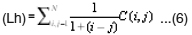
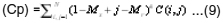
For comparative analysis various other conventional co-occurrence features such as local homogeneity, energy, cluster tendency, cluster
prominence, cluster shade and contrast are estimated from co-occurrence matrix C (i,j), derived from all sub-bands of wavelet decomposition[14].
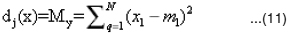
Local homogeneity (Lh)
Cluster Shade (Cs)

Cluster Tendency (Ct) =
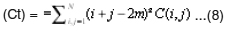
Cluster Prominence (Cp)
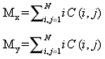
Where
Classification
A training data set is used to train a classifier and another test data set is used to test the classifier. If the features are assumed to have Gaussian density function, Bayes classifier is optimal. Bayes classifier is given by dj(x) = ln P(wj) – ln -{(x – mj)T Cj -1(x-mj)}

Euclidean classifier depends only on the mean positions of the texture classes. Euclidean classifier is given by
In K-NN, the unknown sample data is classified by assigning it the label most frequently represented among the k nearest samples. KNearest Neighbor classifier is given by dj(x)= P(wj|x) if K –nearest neighbors of x are labeled wj

One of the advantages of K-NN is it utilizes the sample data to describe the rules. It also admits noise and does not need any coherence between the samples. The classification time complexity of K-NN is O(n). On the other hand K-NN fails when there are two or more classes which have the same number of nearest neighbor samples. Also it fails when the sample to be classified is isolated and singular. Thus modified K-NN is used to overcome these pitfalls15.
Algorithm for modified K-NN is given below
Let a class Ci ={1,2,….,n) have training
samples xj’={j=1,2,…N} and x be test sample.
Therefore Euclidian distance is given by d (x, xj’).
Take the reciprocal of Euclid distance between the test samples and training samples.
Select k maximum reciprocal of distance of training samples.
Among the k training samples, let Si (i =1,2,..n) be the sum of the reciprocals of distances which belong to class Ci.
Take Si as the class matching degree of class Ci and compare the class matching degree.
If dm(x) = max{Si } (m ª 1,2,…n) , then x ª Cm.
Both the probabilistic and non probabilistic distance measures such as Bayes, Euclidean, and ordinary K-Nearest Neighbor16 are used for comparative study.
Experimental
Experimental evaluation of classification system is carried on the iris images collected from CASIA Iris image Database [V3.0] and MMU Iris Database [MMU04a]. CASIA Iris Image Data base contributes a total number of 756 iris image which were taken in two different time frames and 249 subjects. Each of the iris images is 8-bit gray scale with resolution 320 X 280. MMU data base contributes a total number of 450 iris images which were captured by LG Iris Access→2200. Entire experiment is carried using MATLAB 9.0 and the process involves two phases. One is training phase and the other is classification phase.
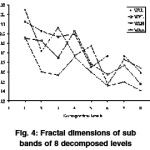
Fractal dimensions of iris template (Flower iris) at different levels of decomposition are shown in Table 1. The best classification rate is achieved at 8 levels with overall performance above 98% a shown in Table 5. Table 3 depicts the variation in accuracy with respect to change in threshold value( 100% and 90% for threshold values of λ= 0 and 0.05 respectively). A comparative study is also performed with conventional statistical features of co-occurrence matrix. The optimal threshold value is set to 0.02 (chosen empirically) to achieve more than 95% accuracy.
Significant co-occurrence features from original images without decomposition which are used for classification in traditional approaches are also shown in Table 4. Table 6 gives the performance of different classifiers when compared with modified K-NN classifier. It is shown that modified K-NN classifier has 100% performance at 8 levels of decomposition and at 6 levels it is 98%. 100 % classification rate is achieved for flower and jewel Sub-bands from Haar wavelet Classified SampleClassifierFeature Vector iris templates due to their rich texture properties while stream and shaker exhibit above 95% classification rates.
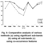 |
Figure 9: Comparative analysis of various methods (a) using significant sub-bands using all sub-bands (c) using co-occurrence features
Click here to View figure
|
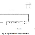
Training Phase
Sixty samples (512 × 512 pixel resolution) are extracted from the above data base.
Each sample is applied to n level Haar wavelet to extract the deterministic patterns.
For each above pattern fractal dimension FD is estimated using box counting method.
Sub-bands with highest FD are used for decomposition to next level.
Decomposition terminates when FD value reaches threshold value λ.
Feature vector is developed using the statistical features of these significant sub-bands.
Steps 2-5 are repeated for all 60 samples and their respective feature vectors are saved in library.
Classification Phase
Feature vector of a new sample that is to be classified is computed as in steps 2-5 of training phase.
A classifier is used to identify the unknown sample.
Steps 1-2 are repeated with three different classifiers such as Bayes, Euclidean and K-NN.
Steps 1-3 are repeated for all 60 samples.
Discussion
A comprehensive algorithm for classification of iris textures based on fractal dimensions and wavelet decomposition has been developed which reduces overheads against exhaustive search and high computational complexities of conventional biometric systems. As non redundant and significant sub-bands are only considered for developing feature space, it is more reliable and reduces time complexity in classification. As the decomposition increases the details in FD will decrease. Thus a proper threshold value must be determined so that there will be an improvement in the reduction of computational time and classification rate.
The exhaustive experiments conducted will bring out a comprehensive approach to classify iris texture even if it is singular or having similar features with other classes. Fractal based wavelet decomposition reduced the size of the feature vector. Usage of modified K-NN results much better classification performance over conventional methods. The overall success rate is improved when 8 levels of decomposed sub-bands are considered. The experiments and results prove the robustness and versatility of algorithm.
Future work includes considering color iris templates for classification by decomposing them initially into R, G and B layers and further considering their significant sub bands.
References
- E. Sreenivasa Reddy, Ch. Subbarao, and I. Ramesh Babu, “Biometric template Classification: A case study in iris textures”, Proceedings of 2nd IEEE International Conference on Biometrics, LNCS4642: 106-1113 (2007).
- J.M. Keller, S. Chen, R.M. Crownover, “Texture description and segmentation through fractal geometry”, Computer Vision and Image Processing and Graphics (1989).
- B. B. Mandelbrot, J.W. Van Ness, “Fractional Brownian motions, fractional noises and applications”, SIAM Rev. 10, 1968.
- Dimitrios Charlampidi and Takis Kasparis, “Rotationally invariant texture segmentation using directional wavelet-based fractal dimensions”, Proc. SPIE, 4391: 115 (2001).
- Aura Conci and Oliveira Nunes, “Multiband Image Analysis using Local Fractal Dimensions”, SIBGRAPI (2002).
- Mona Sharma, Markos Markou, Sameer Singh “Evaluation of Texture Methods for Image Analysis”, pattern recognition letters.
- Lane and J. Fan, “ Texture classification by wavelet packet signatures”, IEEE Transactions, Pattern Analysis and Machine Intelligence.15: 1186-1191 (1993).
- H. O. Peitgen, H. Jurgens, D. Saupe, “Chaos and Fractals: New Frontiers of Science, Springer, Berlin (1992).
- Omar S. AL-Kadi, “ A Fractal Dimension based optimal wavelet Packet analysis technique for classification of Meningioma Brain Tumors” Proceedings of ICIP, 2009, USA.
- S. Arivazhagan, Dr.L. ganesan, S. Deivalakshmi, “ Texture Classification using Wavelet Statistical Features”, Pattern Recognition Letters,24(9-10): 1513-1521(2003).
- Qingmiao Wang, Shinguang Ju, “A Mixed Classifier Based Combination of HMM and KNN”, Proceedings of 4th IEEE International Conference on Natural Computation (2008).
- Karu K, Anil Jain K, and Bolle R M, “Is there any Texture in the Image?”, Journal on Pattern Recognition, Science Direct,29(9):1437-1446 (1996).
- Reed T R and Buf J M H, “A Review of Recent Texture Segmentation and Feature Extraction Techniques,” Computer vision, Image Processing and Graphics Journal,57(3): 359-372 (1993).
- Jill P. Card, J. M. Hyde, and T. Giversen, ‘Discrimination of Surface Textures using Fractal Methods”, Pattern Informatics Publications (2001).
- R.W.Conners and C.A.Harlow, “A theoretical comparison of texture Algorithms”, IEEE transactions on Pattern Analysis and Machine Intelligence,2(3): 204-222(1980).
Views: 104

This work is licensed under a Creative Commons Attribution 4.0 International License.