Navneet* and Nasib Singh Gill 

Maharshi Dayanand University ,Deptt. of Computer Science and Applications, Rohtak Haryana,India

ABSTRACT:

Various attributes within a dataset relate to each other and with the class attribute. The relationship between the different attributes with class attribute may improve the classification accuracy. The paper introduces CCSA algorithm that performs the clustering that is cascaded by classification based on association. The Clustering process generates a group of various instances within the dataset. These clustered instances are classified by using the association. This paper uses the Apriori association to generate the rules for classification. The technique is analyzed by using the soil data set and various other online available datasets using WEKA. The simulation result using the WEKA shows that reduced rules with the improved classification accuracy as compared to the existing association with classification algorithms. 

KEYWORDS: Data mining; PART; WEKA; k-mean clustering; Schwarz criteria; Association

Copy the following to cite this article: Navneet, Gill N. S. A Classification Using the Compact Rule Generation. Orient.J. Comp. Sci. and Technol;8(1)

Copy the following to cite this URL: Navneet, Gill N. S. A Classification Using the Compact Rule Generation. Orient.J. Comp. Sci. and Technol;8(1) Navneet, Gill N. S. A Classification Using the Compact Rule Generation. Orient. J. Comp. Sci. and Technol;8(1). Available from: http://www.computerscijournal.org/?p=1676

Introduction

Data mining is the process to get the hidden information available within the database and it can lead to the knowledge discovery [1][2]. Various operations included in the data mining are the classification, prediction, association and the clustering. The association [3] is most useful application that is used to get the relationship between the elements of particular set. These  properties are based on  co-occurrence of the data items instead of inherent properties of data .Main motive of association is to extract the frequent patterns, associations, casual structures and interesting correlations among various set of items of different transactions of databases or data repositories. Association is mainly applied to the risk management, telecommunication market etc. Association is used to define the relation between various attributes of the active database to get the frequent pattern and the correlation between various set of items within the dataset. This analysis is helpful to get the exact idea of the customer behavior that leads to the progress in business. The number of association rules is large for any given dataset, so association mining [4] is used to get the association rule for a given dataset. In the association mining the dataset is firstly decomposed into the sub sets and this process carries on to get the sets of various items within the dataset. The item sets that exceeds the threshold value is known as large or frequent item set.    Then the association rules are build to derive the relation between various item sets [5].  This paper is further divided in to four sections section 1 describe the association and PART algorithm. The section 2 discusses the related work and the section 3 describes the proposed technique. The section 4 describes the result with their analysis.

Apriori Algorithm

Various association algorithms exist to find the relationship among various attributes of the dataset. Apriori algorithm is found to be the most efficient algorithm among them. The Apriori algorithm completes its process in two steps, first step is to generate the items that has support factor greater than or equal to, the minimum support and the second step is to  generate all rules with confidence factor greater than or equal to the minimum confidence [6]. In the first step,the set of possible itemsets is exponentially increasing that makes the finding of frequent dataset more difficult. The downward closure property is used to find the frequent item sets. The Apriori algorithm find subsets which are common to threshold number of itemsets and uses a “bottom up” approach.  The frequent subsets are extended one item at a time  and groups of candidates are tested against the data. The algorithm terminates when no further successful extensions are found.

Classification Rule Based Part Algorithm

Classification is a concept or process of finding  a model which finds the class of unknown objects. It  basically maps the data items into one of the some  predefined classes[7]. Classification model generate a set of rules based on the features of the data in the training dataset. Further these rules can be used for classification of future unknown data items. Classification is the one of the most important data mining technique. Medical diagnosis is an important application of classification for example, diagnosis of new patients based on their symptoms by using the classification rules about diseases from known cases.

PART stands for Projective Adaptive Resonance  Theory. The input for PART algorithm is the vigilance and distance parameters.

Initialization

Number m of nodes in F1 layer:=number of  dimensions in the input vector. Number m of nodes in F  layer: =expected maximum number of clusters that can be formed at each clustering level.

Initialize parameters L, ρo, ρh, σ, α, θ, and e.

1.Set ρ= ρo.

2.Repeat steps 3 –7 until the stopping condition is satisfied.

3.Set all F2 nodes as being non-committed.

4. For each input vector in dataset S, do steps 4.1-4.6.

4.1 Compute h_ij for all F1 nodes v_i and committed F2 nodes vj. If all F2 nodes are non committed, go to step 4.3.

4.2 Compute T_j for all committed F2 nodes V_j.

4.3 Select the winning F2 node VJ. If no F2 node can  be selected, put the input data into outlier 0 &  then continue to do step 4.

4.4 If the winner is a committed node, compute rJ, otherwise go to step 4.6

4.5 If rJ >=  ρ, go to step 4.6, otherwise reset the winner VJ and go back to step 4.3.

4.6  Set the winner VJ as the committed and update the bottom-up and top-down weights for winner node VJ.

5. Repeat step 4 N times until stable clusters are formed (i.e. until the difference of output clusters say N^th and (N-1)^th time becomes sufficiently small).

6. For each cluster Cj in F2 layer, compute the associated dimension set Dj. Then, set S= Cj and set ρ= ρ+ ρh (or ρ= | D |= ρh), go back to step 2.

7. For the outlier O, set S = 0, go back to step 2.

Related Work

Vamanan. R (2011) [8] finds the suitable model to predict the yield production. The author compares MLR and k-mean clustering technique to determine the average production of the rainfall on the dataset containing the data regarding yearly rainfall in cms by using four parameters i.e. Year, Rainfall, Area of Sowing and Production.  The results are compared with the actual average production then MLR technique gives 96% accuracy while the K-MEAN clustering gives the 98% accuracy. Shweta et al. (2012) [9] have  implemented  clustering  technique  using WEKA  tool  to  create  clusters  of  the  soil  based  on  their salinity. The author creates the cluster to find the relation between the various types of soils in the selected subset of soil. The subset of soil is selected from the world soil science database.  D Ramesh et al. (2013) [10] used k-means approach to estimate the crop yield analysis. They also reviewed various methodologies that are used in agricultural domain and finds Naïve Bayes classifier suitable for the soil classification. Navneet et al. (2014) [11] used Schwarz Criterion (SC) to choose the optimal number of clusters in the k-mean algorithm for a given range of values according to intrinsic properties of the specified data set. Schwarz Criterion is a parametric measure of how well a given model predicts the data. It represents a trade-off between the likelihood of the data for the model and the complexity of the model. The presented algorithm is implemented using the WEKA tool and analyzed on various datasets available at internet. The accuracy of 97.17% is found on the soil dataset.

Ccsa Technique

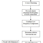
The paper [11] already showed that higher accuracy can be achieved by cascading the clustering with the classification. Moreover, in the paper [11] the technique uses the Schwarz criteria to decide the number of clusters. The technique in the paper [11] gives better results than the existing classification technique. This technique minimizes the classification rules by using the relationship between the attributes instead of gain ratio. The Boolean relation is used to classify the instances.  It can also improve the classification accuracy. In CCSA technique (Cascading of Clustering based on Schwarz criteria and Association) the elements within the dataset are divided in to the number of clusters. The number of clusters within the dataset is determined by the Schwarz criterion. Then the elements within the clusters are classified. The classification occur process determine the frequency of the each class within the clusters. The low frequency component joined with the other components to make a frequent set.  Then the relation is derived between various sets of the clusters. This relation is reduced as the number of sets is reduced due to combining various components in a set. This process is applied to each cluster. The process is explained in the following block diagram.

Figure 1: Block diagram of CCSA Technique   Click here to View figure

 

 The process briefed in the above block diagram can be explained by the following algorithm

CCSA Algorithm

1. Input large Dataset of soil sample.
2. Initiate K=smallest value(default k=2);
3. Apply K-means to generate number of clusters say C0, C1, C2 ,……., Cn.
4. For i=1:n
5. Calculate the Schwarz criterion for cluster Ci by using

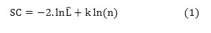
Where  χ= data within the cluster Ci

n= the number elements in Ci

k = the number of parameters to be estimated.

 = The maximized value of the likelihood function of the model M i.e Ĺ= p(x|β)  where     are the parameter values that maximize the likelihood function.

Apply K-mean on Ci Clusters for k=2 say generated Clusters are Ci1 and Ci2

Calculate the SC for Clusters Ci1 and Ci2 by using

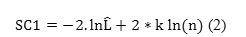
Here, the number of parameters get doubled due to two cluster.

I. If SC>SC1 then n=n+1 i.e. new model preferred.

II. Ci=Ci1 and Cn=Ci2

III. i=i-1

IV. End if

 V. End

 VI. For each cluster

VII. S=elements of Selected Cluster

VIII. I=1

IX. While Li is not empty

X. Se(i+1)=elements generated by Li

XI. For each element in the cluster

XII.Count the candidates of the Se(i+1)

XIII. S(i+1)=candidates of Se(i+1) with minimum support

XIV. End

XV. End

The above process can be implemented by using the WEKA. This process is analyzed on the soil dataset explained in our previous paper. This algorithm is also analyzed on the diabetes and ionosphere dataset. The analysis of these and comparison of results with the PART algorithm and our existing and the kmean clustering with association based classification is done in the next section.

Results and Analysis

The simulation of the CCSA algorithm is done using the WEKA.  The comparison is done between the PART algorithm and the Kmean clustering with association

Rules Generated by the CCSA Techniques are As Follow

pCluster_0_0 > 0.000023 AND

pCluster_1_0 <= 0.000019: MLH (639.0/4.0)

pCluster_2_1 <= 0.571944 AND

pCluster_3_1 <= 0.82491 AND

pCluster_2_0 <= 0.07115 AND

pCluster_3_1 > 0.04404 AND

pCluster_1_0 <= 0.018951 AND

pCluster_4_1 <= 0.000091 AND

pCluster_2_0 <= 0.00588: MLM (311.0/30.0)

pCluster_2_0 <= 0.039564 AND

pCluster_2_1 <= 0.571296 AND

pCluster_4_1 <= 0.003989 AND

pCluster_4_1 <= 0.000052: MLM (506.0/12.0)

pCluster_2_0 > 0.036364: MLM (233.0/29.0)

pCluster_2_1 <= 0.690531 AND

pCluster_4_0 <= 0.000123 AND

pCluster_4_1 > 0.000029 AND

pCluster_4_1 > 0.000091: MLM (28.0)

pCluster_2_1 <= 0.690531 AND

pCluster_4_1 <= 0.003989 AND

pCluster_4_1 <= 0.000029: MLM (172.0/30.0)

pCluster_1_1 <= 0.000028 AND

pCluster_4_1 > 0.006255: MLM (14.0)

pCluster_1_0 <= 0.00001 AND

pCluster_0_1 <= 0.000057 AND

pCluster_2_0 <= 0.015867 AND

pCluster_0_1 <= 0.00001: MLM (7.0/3.0)

pCluster_0_1 > 0.00001 AND

pCluster_0_1 <= 0.000057 AND

pCluster_1_1 <= 0.019452: MLM (6.0/2.0)

pCluster_0_1 <= 0.000024 AND

pCluster_4_0 <= 0.00007: MLL (6.0/1.0)

pCluster_0_1 <= 0.000024 AND

pCluster_1_1 <= 0.008219 AND

pCluster_4_0 > 0.000182: MLH (6.0)

pCluster_0_1 <= 0.000024: MLM (9.0/1.0)

: MLH (4.0)

Rules Generated by the Existing Techniques are As Follow

pCluster_3_0 <= 0.002557 AND

pCluster_1_0 <= 0.000078 AND

pCluster_2_0 <= 0.09236 AND

pCluster_0_2 > 0.000177: MLH (560.0/3.0)

pCluster_0_3 <= 0.206039 AND

pCluster_0_1 <= 0.005072 AND

pCluster_4_0 <= 0.000916 AND

pCluster_2_2 <= 0.568615 AND

pCluster_2_1 <= 0.008903: MLM (529.0/13.0)

pCluster_0_3 <= 0.206039 AND

pCluster_1_3 <= 0.043108 AND

pCluster_0_1 <= 0.002668 AND

pCluster_3_0 > 0.080954 AND

pCluster_3_0 <= 0.485715 AND

pCluster_4_1 <= 0.000811 AND

pCluster_4_0 <= 0.000048 AND

pCluster_2_0 <= 0.007514: MLM (289.0/25.0)

pCluster_0_3 > 0.206039: MLH (80.0/1.0)

pCluster_2_0 > 0.013101 AND

pCluster_2_0 <= 0.462971 AND

pCluster_2_1 > 0.021075 AND

pCluster_3_0 <= 0.319589 AND

pCluster_0_1 > 0.000446 AND

pCluster_2_1 <= 0.048389: MLM (74.0/2.0)

pCluster_2_0 > 0.032287 AND

pCluster_0_1 <= 0.000493 AND

pCluster_4_0 > 0.005655 AND

pCluster_0_1 > 0.000089 AND

pCluster_3_0 <= 0.040292: MLM (69.0/7.0)

pCluster_4_3 > 0.014222 AND

pCluster_4_0 <= 0.032689: MLM (28.0/1.0)

pCluster_4_3 <= 0.014803 AND

pCluster_2_0 <= 0.03813 AND

pCluster_3_0 <= 0.487121 AND

pCluster_1_2 > 0.002153 AND

pCluster_1_1 <= 0.000222: MLM (25.0)

pCluster_2_0 > 0.245194 AND

pCluster_3_3 <= 0.008706 AND

pCluster_4_1 > 0.001556: MLM (29.0/5.0)

pCluster_4_1 <= 0.000966 AND

pCluster_2_0 > 0.034883: MLM (29.0/8.0)

pCluster_2_0 > 0.245194: MLL (7.0/1.0)

pCluster_3_0 > 0.487121 AND

pCluster_3_0 <= 0.487819: MMM (3.0)

pCluster_1_2 <= 0.000969 AND

pCluster_1_0 <= 0.002891 AND

pCluster_0_1 <= 0.011: MLM (159.0/29.0)

pCluster_3_3 > 0.005132 AND

pCluster_1_1 <= 0.000126: MLH (3.0)

pCluster_3_3 <= 0.005132 AND

pCluster_1_0 > 0.003551 AND

pCluster_1_1 <= 0.000033 AND

pCluster_3_2 <= 0.010386: MLM (7.0)

pCluster_0_1 <= 0.001067 AND

pCluster_3_3 <= 0.005132 AND

pCluster_3_3 <= 0.002324 AND

pCluster_1_3 <= 0.000021: MLM (4.0/1.0)

pCluster_3_3 <= 0.005132 AND

pCluster_1_0 > 0.004741 AND

pCluster_0_1 <= 0.000568: MLM (2.0)

pCluster_3_3 <= 0.005132 AND

pCluster_1_0 <= 0.004741 AND

pCluster_1_1 <= 0.00268 AND

pCluster_3_3 <= 0.002324 AND

pCluster_1_1 > 0.000012 AND

pCluster_1_0 <= 0.002296 AND

pCluster_0_1 > 0.011592: MLM (12.0/1.0)

pCluster_0_1 <= 0.001044 AND

pCluster_3_0 <= 0.333462: MLL (4.0)

pCluster_1_1 <= 0.00268 AND

pCluster_3_3 <= 0.002324 AND

pCluster_1_2 <= 0.000043 AND

pCluster_1_1 <= 0.000013 AND

pCluster_3_2 > 0.00004 AND

pCluster_0_1 <= 0.016079: MLM (6.0/2.0)

pCluster_1_3 > 0.014494: MLH (7.0/1.0)

pCluster_3_3 <= 0.002324 AND

pCluster_1_1 <= 0.000036 AND

pCluster_2_1 <= 0.020821 AND

pCluster_1_0 > 0.000093: MLM (5.0)

pCluster_1_1 <= 0.000033: MLH (5.0/1.0)

: MLM (5.0)

Rules Generated by the PART Techniques are As Follow

Village <= 81: MLH (640.0/4.0)

srno > 106 AND

Village > 104 AND

Village <= 241 AND

Block <= 447 AND

potash > 1 AND

Village <= 154 AND

srno > 150: MLM (350.0/7.0)

srno > 104 AND

Village > 152 AND

Village <= 242 AND

potash > 1 AND

Block <= 447 AND

Village > 155 AND

Village <= 180: MLM (189.0/7.0)

srno > 97 AND

Village > 181 AND

Village <= 242 AND

potash > 1 AND

phos <= 1 AND

Village <= 234 AND

Village <= 212 AND

Village > 185 AND

Block <= 447 AND

Village <= 201 AND

Village > 190: MLM (84.0)

srno > 95 AND

potash <= 1: MLM (56.0/1.0)

srno > 95 AND

Village <= 131 AND

potash <= 2 AND

Village > 86 AND

Village > 95 AND

Village <= 103 AND

Village <= 100: MLM (33.0)

srno > 95 AND

Village <= 131 AND

potash <= 2 AND

Village <= 86: MLM (31.0/1.0)

Village > 104 AND

Village <= 242 AND

Block > 447 AND

phos <= 1 AND

Village > 229 AND

Village > 234: MLM (57.0)

Village > 104 AND

Village <= 243 AND

Block > 447 AND

Village <= 215 AND

Village <= 214 AND

Village <= 212: MLM (48.0)

Village > 104 AND

Village <= 243 AND

Block > 447 AND

Village > 215 AND

Village > 218 AND

Village <= 233 AND

Village <= 227: MLM (68.0/3.0)

Village <= 131 AND

potash <= 2 AND

Village > 87 AND

Village > 90 AND

Village > 101: MLM (44.0/6.0)

Village <= 95 AND

Village <= 94 AND

Village > 87 AND

Village <= 90: MLM (24.0)

srno > 91 AND

Village <= 95 AND

Village <= 94 AND

Village > 91: MLM (24.0)

Village <= 95 AND

potash <= 2 AND

srno <= 938: MLH (17.0)

Village <= 243 AND

Village > 181 AND

Village <= 189 AND

Village > 185: MLM (32.0)

Village <= 243 AND

Village > 181 AND

Village > 228 AND

Village <= 233: MLM (35.0)

Village <= 243 AND

Village > 181 AND

Village <= 217 AND

Village > 184 AND

Village > 202 AND

Block <= 447: MLM (25.0)

Village <= 243 AND

Block <= 447 AND

Village <= 98 AND

potash > 2: MLM (10.0)

Village <= 243 AND

Village > 181 AND

Village <= 184: MLM (18.0)

Village <= 243 AND

Village <= 98 AND

srno > 1181: MLH (9.0/3.0)

Village <= 243 AND

Block <= 447 AND

phos <= 1 AND

srno <= 148 AND

srno > 135: MLM (13.0/1.0)

Village <= 243 AND

Block <= 447 AND

phos <= 1 AND

potash <= 2 AND

Village > 187 AND

Village > 196: MLL (8.0/1.0)

Village <= 243 AND

Village <= 183 AND

phos <= 1 AND

potash <= 2 AND

srno > 747 AND

srno > 1062: MLL (13.0/4.0)

Village > 243: MLH (8.0/1.0)

phos > 1 AND

Block > 447 AND

Village > 215 AND

srno > 580 AND

srno > 1071: MLM (3.0/1.0)

phos > 1 AND

Block <= 447: MLH (2.0/1.0)

Block <= 447 AND

potash <= 2 AND

srno <= 669 AND

Village <= 183: MLL (11.0/1.0)

Village <= 215 AND

Village <= 214 AND

Block > 447 AND

Village > 213: MLM (8.0)

Village <= 215 AND

Block > 447 AND

srno <= 1426 AND

Village <= 214: MLM (6.0)

Village <= 215 AND

Block <= 447 AND

Village <= 187: MLM (15.0/6.0)

Block <= 447 AND

srno <= 1523 AND

srno <= 796: MLM (3.0/1.0)

Village <= 215 AND

Block > 447: MMM (10.0/2.0)

Village <= 223 AND

srno > 1415: MLM (7.0)

Block > 447 AND

Village > 238: MLM (8.0)

srno <= 460: MLM (7.0/1.0)

Block > 447 AND

phos <= 1 AND

Village > 231 AND

srno <= 1567: MLL (5.0/1.0)

Village <= 223 AND

Block > 447 AND

Village > 217: MLL (4.0)

Block > 447 AND

phos <= 1 AND

Village <= 231 AND

Village > 222: MMM (6.0/3.0)

Village <= 216: MLL (6.0/1.0)

: MLM (4.0/1.0)

The performance of the algorithm can be measured by using various parameters like TP rate, FP rate, recall, etc. True positive rate (TP rate) is the number of instance belongs to same class as specified by the algorithm divided by the total number of instance. False-positive rate (FP rate) is the number of instance doesn’t belong to the class specified by the algorithm divided by the total number of instances. Precision is the probability that randomly selected instance is correctly classified that can be given as Precision TP/ TP+ PPX 100%.

Recall is the average of probabilities of all instances within dataset. TP/TP + FN X100%. F-measure is mean of precision and the recall can be given as F- measure = 2*precision* recall /precision+ recall.

Table 1: Comparison of Various algorithms using various parameters  Click here to View table

 

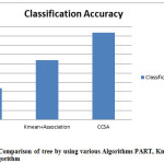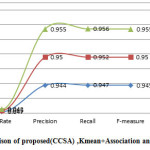
Figure2: Accuracy Comparison of tree by using various Algorithms PART, Kmean+ Association and proposed(CCSA)  algorithm   Click here to View figure

 

Figure3: Comparison of proposed(CCSA),Kmean+Association and PART algorithm   Click here to View figure

 

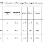
Table 1 shows the comparison among PART,  k-mean + Association and the proposed CCSA algorithm. The classification accuracy and no. of rules of the proposed algorithm is better than the other algorithms..Overall a tree having compact rule and greater classification accuracy is generated by the proposed algorithm. Figure 2 and figure 3 shows the graphical comparison of accuracy  as well as other parameters for PART,  k-mean + Association and the proposed CCSA algorithm. The algorithm can be compared on other datasets. Various datasets are downloaded that are available with WEKA are used to verify the performance of the proposed algorithm. The datasets used are diabetes and the ionosphere. Table 2 specifies various characteristics and performance comparison of the different algorithm on these  datasets.

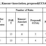Table 2: Comparison of PART, Kmean+Association, proposed(CCSA) algorithms on different datasets.  Click here to View table

 

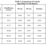
Table 3 shows the proposed algorithm gives No. of rules generated as well as the higher classification accuracy for soil dataset.

Table 3: Comparison of various algorithms on Soil dataset.   Click here to View table

 

The table 3 shows the comparison of the various algorithms on the soil dataset. It can be seen no. of rules are reduced and classification accuracy as well as the TP rate of the proposed algorithm i.e. Schwarz based Kmean clustering cascaded by association based classification is higher than all the other techniques. The number of rules in the PART algorithm is 40 i.e. maximum while in the proposed algorithm is only 13. This shows the reduction in rules. 

Conclusion

The paper produces an algorithm that results in reduced decision rules for classification. The algorithm is developed by cascading the clustering and association based classification algorithm. In the first step the SC (Schwarz Criterion) is applied to get the optimal number of clusters in the KMEAN clustering that is cascaded by association to get the decision tree. The algorithm is implemented using WEKA on the soil data set and two other datasets, and the result shows improved classification accuracy. The number of rules also compared to show the reduction in the rules. Various parameters like TP rate, FP rate, precision, recall, and f-measure are also evaluated to analyze the performance of the proposed algorithm.  In future, the decision tree generating rules can be optimized and other recommendations can extended to other crops of different seasons.

References

1. Dunham, M. H., Xiao, Y., Gruenwald, L., & Hossain, Z. (2001). A survey of association rules. Retrieved January, 5, 2008.
2. Usama M. Fayyad, Gregory Piatetsky-Shapiro, and Padhraic Smyth, From Data Mining to knowledge Discovery: An Overview, Advances in Knowledge Discovery and Data Mining, Edited by Usama M. Fayyad, Gregory Piatetsky-Shapiro, Padraic Smyth, and Ramasamy Uthurusamy, AAAI Press, 1996, pp 1-34.
3. Rakesh Agrawal, Tomasz Imielinski, and Arun N. Swami, Mining Association Rules Between Sets of Items in Large Databases, Proceedings of the 1993 ACM SIGMOD International Conference on Management of Data, pp. 207-216, Washington, D.C., May 1993.
   CrossRef
4. Qureshi, Z., Bansal, J., & Bansal, S. (2013). A survey on association rule mining in cloud computing. International Journal of Emerging Technology and Advanced Engineering, 3(4), 318-321
5. Kotsiantis, S., & Kanellopoulos, D. (2006). Association rules mining: A recent overview. GESTS International Transactions on Computer Science and Engineering, 32(1), 71-82.
6. Divya Bansal, “Execution of APRIORI Algorithm of Data Mining Directed Towards Tumultuous Crimes Concerning Women”, International Journal of Advanced Research in  Computer Science and Software Engineering, Volume 3, Issue 9, September 2013, pp.54-62.
7. Pandey, K., Pandey, P., & KL Jaiswal, A. (2014). Classification Model for the Heart Disease Diagnosis. Global Journal of Medical Research, Volume 14 Issue 1.
8. Ramesh, V., & Ramar, K. (2011). Classification of Agricultural Land Soils: A Data Mining Approach. Agricultural Journal, 6(3), 82-86.
   CrossRef
9. Taneja, S., Arora, R., & Kaur, S. (2012). Mining of Soil Data Using Unsupervised Learning Technique. International Journal of Applied Engineering Research, 7(11), 2012.
10. Ramesh, D., & Vardhan, B. V. (2013). Data Mining Techniques and Applications to Agricultural Yield Data. International Journal of Advanced Research in Computer and Communication Engineering, 2(9).
11. Navneet, N., & Singh Gill, N. (2014). Algorithm for Producing Compact Decision Trees for Enhancing Classification Accuracy in Fertilizer Recommendation of Soil. International Journal of Computer Applications, 98(2), 8-14.
    CrossRef

---

This work is licensed under a Creative Commons Attribution 4.0 International License.